A Future History of Biomedical Progress
The apparent rate of biomedical progress has never been greater.
On the research front, every day more data are collected, more papers published, and more biological mechanisms revealed.
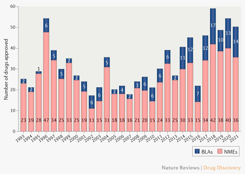
On the clinical front, the pace is also rapid: the FDA is approving more novel therapeutics than ever before, buoyed by a record number of biologics approvals. A flurry of new therapeutic modalities—gene therapies, cell therapies, RNA vaccines, xenogeneic organ transplants—are slated to solve many hard-to-crack diseases over the coming decade.
It seems we are finally on the cusp of ending biomedical stagnation.
Unfortunately, this account isn’t quite correct. Though basic biological research has accelerated, this hasn’t yet translated into commensurate acceleration of medical progress. Despite a few indisputable medical advances, we are, on the whole, still living in an age of bio-medical stagnation.
That said, I’ll make a contrarian case for definite optimism: progress in basic biology research tools has created the potential for accelerating medical progress; however, this potential will not be realized unless we fundamentally rethink our approach to biomedical research. Doing so will require discarding the reductionist, human-legibility-centric research ethos underlying current biomedical research, which has generated the remarkable basic biology progress we have seen, in favor of a purely control-centric ethos based on machine learning. Equipped with this new research ethos, we will realize that control of biological systems obeys empirical scaling laws and is bottlenecked by biocompute. These insights point the way toward accelerating biomedical progress.
Outline
The first half of the essay is descriptive:
Part 1 will outline the biomedical problem setting and provide a whirlwind tour of progress in experimental tools—the most notable progress in biomedical science over the past two decades.
Part 2 will touch on some of the evidence for biomedical stagnation.
Part 3 will recast the biomedical control problem as a dynamics modeling problem. We’ll then step back and consider the spectrum of research ethoses this problem can be approached from, drawing on three examples from the history of machine learning.
The second half of the essay is more prescriptive, looking toward the future of biomedical progress and how to hasten it:
Part 4 will explain the scaling hypothesis of biomedical dynamics and why it is correct in the long-run.
Part 5 will explain why biocomputational capacity is the primary bottleneck to biomedical progress over the next few decades. We’ll then briefly outline how to build better biocomputers.
Part 6 will sketch what the near- and long-term future of biomedical research might look like, and the role non-human agents will play in it.
Niche, Purpose, and Presentation
There are many meta-science articles on why ideas are (or are not) getting harder to find, new organizational and funding models, market failures in science, reproducibility and data-sharing, bureaucracy, and the NIH. These are all intellectually stimulating, and many have spawned promising real-world experiments that will hopefully increase the rate of scientific progress.
This essay, on the other hand, is more applied macro-science than meta-science: an attempt to present a totalizing, object-level theory of an entire macro-field. It is a swinging-for-the-fences, wild idea—the sort of idea that seems to be in relatively short supply. (Consider this a call for similarly sweeping essays written about other fields.) However, because this essay takes on so much, the treatment of some topics is superficial and at points it will likely seem meandering.
All that said, hopefully you can approach this essay as an outsider to biomedicine and come away with a high-level understanding of where the field has been, where it could head, and what it will take to get there. My aim is to abstract out and synthesize the big-picture trends, while simultaneously keeping things grounded in data (but not falling into the common trap of rehashing the research literature without getting to the heart of things, which in the case of biomedicine typically results in naive, indefinite optimism).
1. The Biomedical Problem Setting and Tool Review
Biomedical research is intimidating. At first glance, it seems to span so many subjects and levels of analysis as to be beyond general description. Consider all the subject areas on bioRxiv—how can one speak of the effect of cell stiffness on melanoma metastasis, the evolution of sperm morphology in water fleas, and barriers to chromatin loop extrusion in the same breath? Furthermore, research is accretive and evolving, the frontier constantly advancing in all directions, so this task becomes seemingly more intractable with time.
That said, biomedical research does not defy general description. Though researchers study thousands of different phenomena (as attested to by the thousands of unique research grants awarded by the NIH every year), the scales of which range from nanometers to meters, underneath these particularities lies a unified biomedical problem setting and research approach:
The purpose of biomedicine is to control the state of biological systems toward salutary ends. Biomedical research is the process of figuring out how to do this.
Biomedical research has until now been approached predominantly from a single research ethos.
By “research ethos”, I do not quite mean culture. Rather, I mean the guiding values that (often subconsciously) suffuse all aspects of a research enterprise, the imperceptible cognitive scaffolding that cultural practices are built around.
This ethos aims to control biological systems by building mechanistic models of them that are understandable and manipulable by humans (i.e., human-legible). Therefore, we will call this dominant research ethos the “mechanistic mind”.
The history of biomedical research so far has largely been the story of the mechanistic mind’s attempts to make biological systems more legible. Therefore, to understand biomedical research, we must understand the mechanistic mind.
Tools of the Mechanistic Mind
The mechanistic mind builds models of biology by observing and performing experiments on biological systems. To do this, it uses experimental tools.
Because they are the product of the mechanistic mind, these tools have evolved unidirectionally toward reductionism. That is, these tools have evolved to carve and chop biology into ever-smaller conceptual primitives that the mechanistic mind can build models over.
We’d like to understand how the mechanistic mind’s models of biology have evolved. However, delving into its particular phenomena of study—specific biological entities, processes, etc.—would quickly bog us down in details.
But we can exploit a useful heuristic: experimental tools determine the limits of our conceptual primitives, and vice versa. Therefore, we can tell the story of the mechanistic mind’s progress in understanding biology through the lens, as it were, of the experimental tools it has created to do so. By understanding the evolution of these tools, one can understand much of the history of biomedical research.
The extremely brief summary of this evolution goes:
In the second half of the 20th century, biomedical research became molecular (i.e., the study of nucleic acids and proteins). At the turn of the 21st century, with the (near-complete) sequencing of the human genome, molecular biology became computational. The rest is commentary.
Scopes, Scalpels, and Simulacra
That summary leaves a lot to be desired.
To make further sense of it, we can layer on a taxonomy of experimental tools, composed of three classes: scopes, scalpels, and simulacra.
- “Scopes” are used to read state from biological systems.
- “Scalpels” are used to perturb biological systems.
- “Simulacra” are physical models that act as stand-ins for biological systems we’d like to experiment on or observe but can’t.
This experimental tool taxonomy is invariant across eras and physical scales of biomedical research, generalizing beyond any particular paradigm like cell theory or genomics. These three tool classes are, in a sense, the tool archetypes of experimental biomedical research.
Therefore, to understand the evolution in experimental tools (and, consequently, the evolution of the mechanistic mind), we can simply track advances in these three tool classes. We will pick up our (non-exhaustive) review around 15 years ago, near the beginning of the modern computational biology era, when tool progress starts to appreciably accelerate. (We will tackle scopes and scalpels now and leave simulacra for later.) I hope to convey a basic understanding of how these tools are used to interrogate biological systems, the rate they’ve been advancing at, and the resulting inundation of biomedical data we’ll soon face.
Scopes
To reiterate, scopes are tools that read state from biological systems. But this raises an obvious question: what is biological state?
As alluded to earlier, in the mid-20th century biological research became molecular, meaning it became the study of nucleic acids and proteins. Therefore, broadly speaking, biological state is information about the position, content, interaction, etc. of these molecules, and the larger systems they compose, within biological systems. Subfields of the biological sciences are dedicated to interrogating facets of biological state at different scales—structural biologists study the nanometer-scale folding of proteins and nucleic acids, cell biologists study the orchestrated chaos of these molecules within and between cells, developmental biologists study how these cellular processes drive the emergence of higher-order organization during development, and so on.
Regardless of the scale of analysis, advances in tools for reading biological state (i.e., scopes) occur along a few dimensions:
-
feature-richness
-
spatio-temporal resolution
-
spatio-temporal extent
-
throughput (as measured by speed or cost)
However, there are tradeoffs between these dimensions, and therefore they map out a scopes Pareto frontier.
In the past two decades, we’ve seen incredible advances along all dimensions of this frontier.
To illustrate these advances, we will restrict our focus to the evolution of three representative classes of scopes, each of which highlights a different tradeoff along this frontier:
-
extremely feature-rich single-cell methods
-
spatially resolved methods, which have moderate-to-high feature richness and spatio-temporal resolution
-
light-sheet microscopy, which has large spatio-temporal extent, high spatio-temporal resolution, and low feature-richness
By tracking the evolution of these methods over the past two decades, we’ll gain an intuition for the rate of progress in scopes and where they might head in the coming decades.
But we must first address the metatool which has driven many, but not all, of these advances in scopes: DNA sequencing.
Sequencing as Scopes Metatool
DNA sequencing is popularly known as a tool for reading genetic sequences, like an organism’s genome. But lesser known is the fact that sequencing can be indirectly used to read many other types of biological state. You can therefore think of sequencing as a near-universal solvent or sensor of the scopes class—much progress in scopes has simply come from discovering how to cash out different aspects of biological state in the language of A’s, T’s, G’s and C’s.
The metric of sequencing progress to track is the cost per gigabase ($/Gb): the cost of consumables for sequencing 1 billion base pairs of DNA. Bioinformaticians can fuss about the details—error rates, paired-end vs. single-read, throughput, read quality in recalcitrant regions of the genome like telomeres or repetitive stretches—but for our purposes this metric provides the single best index of progress in sequencing over the past two decades.
For a thorough history of sequencing, see this review article.
You’ve probably seen the famous NIH sequencing chart, which plots the cost per Mb of sequencing (1000 Mb equals 1 Gb). However, this chart is somewhat confusing—the curve clearly appears piecewise linear, with steady Moore’s-law-esque progress from 2001 to 2007, then a period of rapid cost decline from mid-2007 to around 2010, followed by a seeming reversion to the earlier rate of decline.

For the purposes of extrapolation, the current era of sequencing progress started around 2010 (when Illumina released the first in its line of HiSeq sequencers, the HiSeq2000). When we plot sequencing prices from then onward, restricting ourselves to short-read methods, we get the following plot.
Plotted are the cheapest sequencing consumables prices available by year, stratified by device throughput class (which reflects the cost of the sequencing instrument). All data points are the minimum price available that year for a given read length class and throughput class, but note that some cost estimates in the 2010-2015 period were difficult to verify, and therefore multiple prices are given.

Over the past 12 years, the price per gigabase on high-volume, short-read sequencers has declined by almost two orders of magnitude, halving roughly every 2 years—slightly slower than Moore’s law.
Granted, if we measured over the past 15 years, starting with the original Solexa technology that Illumina acquired and commercialized, which allegedly could sequence 1 Gb for $1000-$3000 in 2007 and for $400 in 2009 (per Illumina’s marketing materials), then the trend would appear basically on par with Moore’s law.
The first order of magnitude cost decline came in the 2010-2015 period with Illumina’s HiSeq line, the price of sequencing plummeting from ~$100/Gb to ~$10/Gb; this was followed by 5 years of relative stagnation, for reasons unknown; and in the past 2 years, there’s been another order of magnitude drop, with multiple competitors finally surpassing Illumina and approaching $1/Gb prices. The sequencing market is starting to really heat up, and that likely means the biennial doubling trend will hold; if it does, and if current prices are to be believed, then we can expect sequencing prices to hit $0.1/Gb around 2028-2029.
To make this trend more intuitive, we can explain it in terms of the cost of sequencing a human genome.
A haploid human genome (i.e., one of the two sets of 23 chromosomes the typical human has) is roughly 3 Gb (bases, not bytes) on average (e.g., the X chromosome is much larger than the Y chromosome, so a male’s two haploid genomes will differ in size). Therefore, sequencing this haploid genome at 30x coverage—meaning each nucleotide is part of (i.e., covered by) 30 unique reads on average—which is the standard for whole genome sequencing, results in ~90 Gb of data (call it 100 Gb to make the numbers round). So, we can use this 100 Gb human genome figure as a useful unit of measurement for sequencing prices.
In 2010 to 2011, a human genome cost somewhere in the $5,000 to $50,000 range; by 2015, the price had fallen to around $1000; and now, in 2022, it is allegedly nearing $100 (though this was already being claimed two years ago).
This exponential decline in price has led to a corresponding exponential increase in genome sequencing data. Since around 2014, the number of DNA bases added per release cycle to GenBank, the repository of all publically available DNA sequences, has doubled roughly every 18 months.


But as noted earlier, sequencing has many uses other than genome sequencing. Arguably, the revolution in reading non-genomic biological state has been the most important consequence of declining sequencing costs.
The Single-Cell Omics Revolution
Biological systems run off of nucleic acids and proteins, among other macromolecules. And because proteins are translated from RNA, all biological complexity ultimately traces back to the transformations of nucleic acids—epigenetic modification of DNA, transcription of DNA to RNA, splicing of RNA, etc. Sequencing-based scopes allow us to interrogate these nucleic acid-based processes.
We can divide the study of these processes into two areas: transcriptomics, the study of RNA transcripts, which are transcribed from DNA; and epigenomics, the study of modifications made to genetic material above the level of the DNA sequence, which can alter transcription.
Transcriptomics and epigenomics have been studied for decades. However, the past decade was an incredibly fertile period for these subjects due to the combination of declining sequencing costs and advances in methods for preparing biological samples for sequencing-based readout.
The defining feature of these sample preparation methods has been their biological unit of analysis: the single cell.
It’s not inaccurate to call the past decade of computational biology the decade of single-cell methods. The ability to read epigenomic and transcriptomic state at single-cell resolution has revolutionized the study of biological systems and is the source of much current biomedical optimism.
Applications of Single-Cell Omics
To understand how much single-cell methods have taken off, consider the following chart:

This is a plot of the number of cells in each study added to the Human Cell Atlas, which aims to “create comprehensive reference maps of all human cells—the fundamental units of life—as a basis for both understanding human health and diagnosing, monitoring, and treating disease.” The number of cells per study has been increasing by an order of magnitude a little under every 3 years—and the frequency with which studies are added is increasing too.
The HCA explains their immense ambitions like so:
Cells are the basic units of life, but we still do not know all the cells of the human body. Without maps of different cell types, their molecular characteristics and where they are located in the body, we cannot describe all their functions and understand the networks that direct their activities.
The Human Cell Atlas is an international collaborative consortium that charts the cell types in the healthy body, across time from development to adulthood, and eventually to old age. This enormous undertaking, larger even than the Human Genome Project, will transform our understanding of the 37.2 trillion cells in the human body.
The way these human cells are charted is by reading out their internal state via single-cell methods. That is, human tissues (usually post mortem, though for blood and other tissues this isn’t always the case) are dissociated into individual cells, and then these cells’ contents are assayed (i.e., profiled, or read out) along one or more dimensions of transcriptomic or epigenomic state.
Crucially, these assays rely on sequencing for readout. In the case of single-cell RNA sequencing, the RNA transcripts inside the cells are reverse transcribed into complementary DNA sequences, which are then read out by sequencers. But sequencing can be used to read out other types of single-cell state that aren’t natively expressed in RNA or DNA—chromatin conformation, chromatin accessibility, and other epigenomic modifications—which typically requires a slightly more convoluted library preparation.
The upshot is that these omics profiles, as they are called, act as proxies for the cells’ unique functional identities. Therefore, by assaying enough cells, one can develop a “map” of single-cell function, which can be used to understand the behavior of biological systems with incredible precision. Whereas earlier bulk assays lost functionally consequential inter-cellular heterogeneity in the tissue-average multicellular soup, now this heterogeneity can be resolved in its complete, single-cell glory. These single-cell maps look like so (this one is of a very large human fetal cell atlas, which you can explore here):

And the Human Cell Atlas is the tip of the iceberg—single-cell omics methods have taken the entire computational biology field by storm. These methods have found numerous applications: comparing cells from healthy and diseased patients; tracking the differentiation of a particular cell type to determine the molecular drivers, which might go awry in disease; and comparing single-cell state under different perturbations, like drugs or genetic modifications. Open up any major biomedical journal and you’re bound to see an article with single-cell omics data.
Single-cell methods have become de rigueur in computational biology. Somewhat ironically, the ability to parse biological heterogeneity has driven methodological homogenization of the field. Papers are now rather formulaic, including basically the same types of data, analysis and figures—a dimensionality reduction plot of single-cell profiles (i.e., a “single-cell map”), a volcano plot showing differential gene expression between two conditions, a visualization of the inferred gene regulatory network, and a matrix of gene expression values across pseudotime for key gene regulatory nodes.
Every year or two a fancy new analysis method will come along, which is aped by the entire field: there are more than 70 methods for inferring cellular trajectories on single-cell maps, a dozen methods for inferring cell-cell communication from gene expression data, and a dozen methods and counting for inferring gene regulatory networks. Research has to an extent become paint-by-numbers: do single-cell omics on your biological system of study, apply new single-cell analysis method X to the data, and then tell a compelling mechanistic story about the results.
(Single-cell maps have become so important to the field of computational biology that these maps are now being made accessible to the color-blind.)
But this rapid expansion of single-cell data is only made possible by continual advances in methods for isolating and assaying single cells.
Single-Cell Omic Technologies
Over the past decade or so, single-cell sample preparation methods have advanced along two axes: throughput (as measured by cost and speed) and feature-richness (as measured by how many omics profiles can be assayed at once per cell and the resolution of these assays).
Svensson et al. explain the exponential increase in single-cell transcriptomic throughput over the past decade as the result of multiple technical breakthroughs in isolating and processing single cells at scale:
A jump to ~100 cells was enabled by sample multiplexing, and then a jump to ~1,000 cells was achieved by large-scale studies using integrated fluidic circuits, followed by a jump to several thousands of cells with liquid-handling robotics. Further orders-of-magnitude increases bringing the number of cells assayed into the tens of thousands were enabled by random capture technologies using nanodroplets and picowell technologies. Recent studies have used in situ barcoding to inexpensively reach the next order of magnitude of hundreds of thousands of cells.

That is, once a tissue has been dissociated into single cells, the challenge then becomes organizational: how do you isolate, process, and track the contents of these cells? In the case of transcriptomics, at some point the contents of the cell must undergo multiple steps of library preparation to transform RNA transcripts into DNA, and then these DNA fragments must be exposed to the sequencer for readout—all without losing track of which transcript came from which cell.
As can be seen in the graph, throughput began to really take off around 2013. But these methods have continued to advance since the above graph was published.
For instance, combinatorial indexing methods went from profiling 50,000 nematode cells at once in 2017, to profiling two million mouse cells at once in 2019, to profiling (the gene expression and chromatin accessibility of) four million human cells at once in 2020. With these increases in scale have come corresponding decreases in price per cell—even in the past year, sci-RNA-seq3, the most recent in this line of combinatorial indexing methods, was further optimized, making it ~4x less expensive than before, nearing costs of $0.003 per cell at scale.
Costs have also declined among commercial single-cell preparation methods. 10X Genomics, the leading droplet-based single-cell sample preparation company, offers single-cell RNA sequencing library preparation at a cost of roughly $0.5 per cell. But Parse Biosciences, which, like sci-RNA-seq3, uses combinatorial indexing, recently claimed its system can sequence up to a million cells at once for only $0.09 per cell. (Though one can approach these library preparation prices on a 10x chip by craftily multiplexing and deconvoluting—that is, by labeling cells from different samples, multiple cells can be loaded into the same droplet, and the droplet readout can be demultiplexed (i.e., algorithmically disentangled) after the fact, thereby dropping the cost per cell.)
Thus, like with sequencing, there’s an ongoing gold-rush in single-cell sample preparation methods, and commercial prices should only decline further—especially given that the costs of academic methods are already an order of magnitude lower.
The second dimension along which single-cell methods have progressed in the richness of their readout.
In the past few years, we’ve seen an efflorescence of so-called “multi-omic” methods, which simultaneously profile multiple omics modalities in a single-cell. For instance, one could assay gene expression along with an epigenomic modality, like chromatin accessibility, and perhaps even profile cellular surface proteins at the same time. The benefit of multi-omics is that different modalities share complementary info; often this complementary information aids in mechanistically interrogating the dynamics underlying some process—e.g., one can investigate if increases in chromatin accessibility near particular genes precede upregulation of those genes.
Yet not only can we now profile more modalities simultaneously, but we can do so at higher resolution. To give a particularly incredible example, the maximum resolution of (non-single-cell) sequencing-based chromatin conformation assays went from 1 Mb in 2009, to ~5 kb in 2020, to 20 base pairs in 2022—an increase in resolution of over four orders of magnitude. Since we’re nearing the limits of resolution, future advances will likely come from sparse input methods, like those that profile single cells, and increased throughput.
Thus, improvements in sequencing and single-cell sample preparation methods have revolutionized our ability to read out state from biological systems.
But as great as single-cell methods are, their core limitation is non-existent spatio-temporal resolution. That is, because these methods require destroying the sample, we get only a snapshot of cellular state, not a continuous movie—the best we can do is reconstructing pseudo-temporal trajectories after the fact based on some metric of cell similarity (which is perhaps one of the most influential ideas in the past decade of computational biology), though some methods are attempting to address this temporal limitation. And because we dissociate the tissue before single-cell sample preparation, all spatial information is lost.
However, this latter constraint is addressed by a different set of scopes: spatial profiling methods.
Spatial Profiling Techniques
If single-cell omics methods defined the 2010’s, then spatial profiling methods might define the early 2020’s. These methods readout nucleic acids along with their spatial locations. This information is valuable for obvious reasons—cells don’t live in a vacuum, and spatial organization plays a large role in multicellular interaction.
We’ll briefly highlight two major categories of these methods: sequencing-based spatial transcriptomics, which resolve spatial location via sequencing, and fluorescence in situ hybridization (FISH) approaches, which resolve spatial location via microscopy.
For a more thorough treatment of spatial profiling techniques, see the Museum of Spatial Transcriptomics.
Sequencing-Based Spatial Transcriptomics
The premise of sequencing-based spatial transcriptomics is simple: rather than randomly dissociating a tissue before single-cell sequencing, thereby losing all spatial information, RNA transcripts can be tagged with a “barcode” based on their location, which can later be read out via sequencing alongside the transcriptome, allowing for spatial reconstruction of the locations of the transcripts.
These barcodes are applied by placing a slice of tissue on an array covered with spots that have probes attached to them. When the tissue is fixed and permeabilized, these probes capture the transcripts in the cells above them; then, complementary DNA sequences are synthesized from these captured transcripts, with specific spatial barcodes attached depending on the location of the spot. When these DNA fragments are sequenced, the barcodes are read out with the transcripts and used to resolve their spatial positions.
One major dimension of advance of these methods is spatial resolution, as measured by the size of the spots which RNA transcripts bind to, which determines how many cells are mapped to a single spot, and therefore the resolution with which gene expression can be resolved. Over just the past 3 years, maximum resolution has jumped by almost three orders of magnitude (image source):

These spatial transcriptomics methods produce stunning images. For instance, here’s a section of the developing mouse brain as profiled by the currently highest resolution method, Stereo-seq:

Each dot in the middle pane represents the intensity of the measured gene at that location, but plots of this sort can be generated for all the tens of thousands of genes assayed via RNA sequencing. In the left pane, these complete gene expression profiles are used to assign each dot to its predicted average cell-type cluster, as one might do with non-spatial single-cell transcriptomics.
Yet note the resolution in the rightmost pane of the above figure—it is even greater than that of the middle pane. This image uses in situ hybridization, the basis of the spatial profiling technique we’ll explore next.
smFISH
Fluorescent in situ hybridization (FISH) methods trade off feature-richness for increased spatial resolution. That is, FISH-based methods don’t assay the RNA of every single protein-coding gene like sequencing-based methods do, but in return they localize the transcripts they do assay better.
Instead of using sequencing for readout, these methods use the other near-universal solvent or sensor of the scopes class: microscopy.
That is, whereas spatial transcriptomics resolve the location of transcripts indirectly via sequencing barcodes, FISH methods visually resolve location via microscopy. They do this by repeatedly hybridizing (i.e., binding) complementary DNA probes to targeted nucleic acids in the tissue (attached to these probes are fluorophores which emit different colors of light); after multiple rounds of hybridization and fluorescent emission from these probes, the resulting multi-color image can be deconvolved, the “optical barcodes” used to localize hundreds of genes at extremely high spatial resolution.
Unlike spatial transcriptomics, which is a hypothesis-free method that doesn’t (purposefully) select for particular transcripts, in FISH the genes to probe must be selected in advance, and typically they number in the tens or hundreds, not the tens of thousands like with spatial transcriptomics (though in principle they can reach these numbers—see below). The number of genes that can be resolved per sample (i.e., multiplexed) is limited by the size and error-rates of the fluorescent color palette that is used to mark them, and the spatial resolution with which these transcripts are localized is limited by the sensor’s ability to distinguish these increasingly crowded fluorescent signals (perhaps so crowded that the distance between them falls beneath the diffraction limit of the sensor).
The general idea of FISH has been around for over 50 years, but the current generation of multi-gene single-molecule FISH (smFISH) methods only began to take off around 15 years ago. Since then, there’s been a fair deal of progress in gene multiplexing and the number of cells that can be profiled at once (images source):


But the best way to understand these advances is visually. For instance, we can look at MERFISH, a technique which has been commercialized, part of a growing market for FISH-based spatial profiling methods. Here’s what part of a coronal slice of an adult mouse brain, with more than 200 genes visualized, looks like (the scale-bar is 20 microns in the left pane and 5 microns in the right pane):

The amount of data these methods generate is immense:
As a point of reference, the raw images from a single run of MERFISH for a ~1 cm^2 tissue sample contain about 1 TB of data.
But like spatial transcriptomics, these smFISH methods have one major drawback: though they can spatially resolve extremely feature-rich signals, they lack temporal resolution—that is, they image dead, static tissues, a problem addressed by longitudinal methods like light-sheet microscopy.
Light-Sheet Microscopy
Biological systems operate not only across space, but across time.
Methods like light-sheet fluorescence microscopy (LSFM) trade off feature-richness in exchange for this temporal resolution, all while maintaining high spatial extent and resolution. The niche filled by LSFM is explained as follows:
Fluorescence microscopy in concert with genetically encoded reporters is a powerful tool for biological imaging over space and time. Classical approaches have taken us so far and continue to be useful, but the pursuit of new biological insights often requires higher spatiotemporal resolution in ever-larger, intact samples and, crucially, with a gentle touch, such that biological processes continue unhindered. LSFM is making strides in each of these areas and is so named to reflect the mode of illumination; a sheet of light illuminates planes in the sample sequentially to deliver volumetric imaging. LSFM was developed as a response to inadequate four-dimensional (4D; x, y, z and t) microscopic imaging strategies in developmental and cell biology, which overexpose the sample and poorly temporally resolve its processes. It is LSFM’s fundamental combination of optical sectioning and parallelization that allows long-term biological studies with minimal phototoxicity and rapid acquisition.
That is, LSFM gives us the ability to longitudinally profile large 3D living, intact specimens at high spatial and temporal resolution. Thus, it plays an important complementary role to moderately feature-rich spatial transcriptomic methods and extremely feature-rich single-cell methods, both of which lack temporal resolution.
See this methods primer if you wish to dig into the physics and history behind LSFM.
Needless to say, the technology underlying LSFM has advanced quite a lot over the past two decades. The beautiful thing about spatio-temporally resolved methods is that we can easily witness these advances with our eyes. For instance, we can compare the state of the art in imaging fly embryogenesis in 2004 vs. in 2016:
Yet in just the past year, we have seen further advances still. A new, simplified system has improved imaging speed while maintaining sub-micron lateral and sub-two-micron axial resolution—and on large specimens, no less.
And recently an LSFM method was developed that can image tissues at subcellular resolution in situ, without the need for exogenous fluorescent dyes—in effect, a kind of in vivo 3D histology. The applications of this technology, to both research and diagnostics, are numerous.
You might be asking how one can perform LSFM on in situ tissue if there are no fluorophores to excite. To solve this, the researchers exploit the natural fluorescent emission of some cellular structures, allowing for non-invasive “label-free imaging”—though this method is also compatible with traditional fluorescent dyes, as seen in the video below.
Here’s the stitching together of a 3D-resolved (but not temporally resolved) slice of in situ mouse kidney:
And here’s real-time imaging of a fluorescent tracer dye perfusing mouse kidney tubules in situ:
Granted, both mouse kidney videos required anesthetizing the mouse and opening up its gut so its kidneys could be more directly exposed for imaging, so it’s not exactly noninvasive.
Scopes Redux
The scopes Pareto frontier has advanced tremendously over the past two decades, and on many dimensions at a surprisingly regular rate. This is perhaps the most exciting development in all of biomedical research.
If one had to bet on a particular class of methods that will come to the fore in the next decade, the most underrated bet would be temporally resolved methods like LSFM. As the fine-grain multicellular behavior of large biological systems becomes the object of study beyond developmental biology, we’ll likely see improvements in the throughput, spatio-temporal extent and resolution, and cost of these systems.
However, the ability to read state from biological systems doesn’t alone much improve our understanding of them—for that, we must perturb them.
Scalpels
Scalpels are used to experimentally perturb biological systems. The dimensions of the scalpels Pareto frontier are similar to those of the scopes Pareto frontier:
-
feature precision
-
spatio-temporal precision
-
spatio-temporal extent
-
throughput
However, the past decade has been one dominated by advances in scopes, not scalpels. One metric of this dominance is the annual Nature method of the year, which is a good gauge for what tools are becoming popular among biological researchers. Among the past 15 winners, two are scalpels (optogenetics and genome editing), two are related to simulacra (iPSC and organoids), and the rest are scopes (NGS, super-resolution fluorescence microscopy, targeted proteomics, single-cell sequencing, LSFM, cryo-EM, sequencing-based epitranscriptomics, imaging of freely behaving animals, single-cell multiomics, and spatial transcriptomics) or analytical methods (protein structure prediction).
It’s hard to imagine the counterfactual of wide-ranging progress in scalpels with minimal progress in scopes. This might reflect a deep truth about tool sequencing: reading state from biological systems is a prerequisite to developing the conceptual tools necessary to build the experimental tools that can perturb those systems. For instance, it would be much more difficult to edit a genome if you didn’t understand its physical structure first, which requires imaging it.
Scalpels have simply experienced far narrower progress over the past decade or so than scopes. Advances occurred mostly along the feature-precision and throughput dimensions within a single suite of tools, which we will restrict our attention to (and therefore this section will be comparatively short).
Though the scalpels we review here are useful for interrogating biological dynamics at the level of the cell and below, truly advanced biomedical research will require modeling dynamics at the multicellular level and above. Therefore, we must develop tools for perturbing biological systems at this level, ideally in situ, with high spatial and temporal control—in effect, we must develop the scalpel counterparts to the spatially and temporally resolved scopes that have been developed over the past decades.
Genome and Epigenome Editing
The most notable advance in scalpels has been in our ability to perturb the genome and epigenome with high precision, at scale. Of course, we’re referring to the technology of CRISPR, which researchers successfully appropriated from bacteria a decade ago (though there’s some disagreement about whom the credit should go to).
When one thinks of CRISPR, they likely think about making DNA double-strand breaks (DSB) in order to knock out (i.e., inhibit the function of) whole genes. But CRISPR is a general tool for using guide RNAs to direct nucleases (enzymes which cut DNA or RNA, like the famous Cas9) to specific regions of the genome—in effect, a kind of nuclease genomic homing guidance system. By varying the nuclease one uses and the molecules attached to them, a variety of functions other than knockouts can be performed: targeted editing of DNA without DSB, inhibiting gene expression without DSB, activating gene expression, editing epigenetic marks, and RNA editing and interference.
CRISPR is not the first system to perform most of these functions, and it certainly isn’t perfect—transfection rates are still low and off-target effects still common—but that’s beside the point: the defining features of CRISPR are its generality and ease of use. If sequencing and microscopy are the universal sensors of the scopes tool class, then CRISPR might be the universal genomic actuator of the scalpels tool class.
In conjunction, these scopes and scalpels have enabled interrogating the genome at unprecedented resolution and throughput.
Using Scopes and Scalpels to Interrogate the Genome and Beyond
By perturbing the genome and observing how the state of a biological system shifts, we can infer the mechanistic structure underlying that biological system. Advances in scopes and scalpels have made it possible to do this at massive scale.
For instance, one could use CRISPR to systematically knockout every single gene in the genome across a set of samples (perhaps with multiple knockouts per sample), a so-called genome-wide knockout screen. But whereas previously the readout of these screens was limited to simple phenotypes like fitness (that is, does inhibiting a particular gene produce lethality, which can be inferred by counting the guide RNAs in the surviving samples) or a predefined set of gene expression markers, due to advances in scopes we can now read out the entire transcriptome from every sample.
Over the past five years, a lineage of papers has pursued this sort of (pooled) genome-wide screening with full transcriptional readout at increasing scale. In one of the original 2016 papers, only around 100 genes were knocked out across 200,000 mouse and human cells; yet in one of the most recent papers, all 10,000+ protein-coding genes are inhibited across more than 2.5 million human cells, with full transcriptional readout.
Yet the genome is composed of more than protein-coding genes, and ideally we’d like to systematically perturb non-protein-coding regions, which play an important role in the regulation of gene expression. The usefulness of such screens would be immense:
The human genome is currently believed to harbour hundreds-of-thousands to millions of enhancers—stretches of DNA that bind transcription factors (TFs) and enhance the expression of genes encoded in cis [i.e., on the same DNA strand]. Collectively, enhancers are thought to play a principal role in orchestrating the fantastically complex program of gene expression that underlies human development and homeostasis. Although most causal genetic variants for Mendelian disorders fall in protein-coding regions, the heritable component of common disease risk distributes largely to non-coding regions, and appears to be particularly enriched in enhancers that are specific to disease-relevant cell types. This observation has heightened interest in both annotating and understanding human enhancers. However, despite their clear importance to both basic and disease biology, there is a tremendous amount that we still do not understand about the repertoire of human enhancers, including where they reside, how they work, and what genes they mediate their effects through.
In 2019, the first such massive enhancer inhibition screen with transcriptional readout was accomplished, inhibiting nearly 6,000 enhancers across 250,000 cells, an important step to systematic interrogation of all gene regulatory regions.
But inhibition and knockout are blunt methods of perturbation. To truly understand the genome, we must systematically mutate it. Unfortunately, massively parallel methods for profiling the effects of fine-grain enhancer mutations don’t yet read out transcriptional state at scale, instead opting to trade off readout feature richness for screening throughput via the use of reporter gene assays. However, we’ll likely see fine-grain enhancer mutation screens with transcriptional readout in the coming years.
Yet advances in scopes enable us to interrogate the effects of not only genomic perturbations, but therapeutic chemical perturbations, too:
High-throughput chemical screens typically use coarse assays such as cell survival, limiting what can be learned about mechanisms of action, off-target effects, and heterogeneous responses. Here, we introduce “sci-Plex,” which uses “nuclear hashing” to quantify global transcriptional responses to thousands of independent perturbations at single-cell resolution. As a proof of concept, we applied sci-Plex to screen three cancer cell lines exposed to 188 compounds. In total, we profiled ~650,000 single-cell transcriptomes across ~5000 independent samples in one experiment. Our results reveal substantial intercellular heterogeneity in response to specific compounds, commonalities in response to families of compounds, and insight into differential properties within families. In particular, our results with histone deacetylase inhibitors support the view that chromatin acts as an important reservoir of acetate in cancer cells.
However, though impressive, it’s an open question whether such massive chemical screens (and all the tool progress we’ve just reviewed) will translate into biomedical progress.
2. The End (of Biomedical Stagnation) Is Nigh
Progress in experimental tools over the past two decades has been remarkable. It certainly feels like biomedical research has been completely revolutionized by these tools.
This revolution is already yielding advances in basic science. To name but a few:
-
Our understanding of longevity has advanced tremendously, from the relationship between mutation rates and lifespan among mammals, to the molecular basis of cellular senescence and rejuvenation (which could have huge clinical implications).
-
Open up any issue of Nature or Science and you’re bound to see a few amazing computational biology articles interrogating some biological mechanism with extreme rigor, likely using the newest tools.
-
And how can one forget Alphafold, the solution to a 50-year-old grand challenge in biology. “It will change medicine. It will change research. It will change bioengineering. It will change everything.” (Well, it isn’t necessarily a product of the tools revolution, but it is a major leap in basic science that contributes to the current mood of optimism.)
Biomedical optimism abounds for other reasons, too. Consider some of the recent clinical successes with novel therapeutic modalities:
-
Gene therapy (i.e., genetically edited autologous stem cell transplants) seem poised to solve terrible blood disorders like sickle cell disease and familial hypercholesterolemia.
-
RNA vaccines solved SARS-CoV-2, so maybe they’ll solve other infectious diseases, like HIV. Perhaps they’ll even solve pancreatic cancer. (Or how about the immuno-oncology double-whammy: combining CAR-T and RNA vaccines to treat solid tumors.)
It certainly feels like this confluence of factors—Moore’s-law-like progress in experimental tools, the ever-increasing mountain of biological knowledge they are generating, and a bevy of new therapeutic modalities that are already delivering promising clinical results—is ushering in the biomedical golden-age. Some say that “almost certainly the great stagnation is over in the biomedical sciences.”
How much credence should we give this feeling—are claims of the end of biomedical stagnation pure mood affiliation?
Premature Celebration
A good place to start would be to define what the end of biomedical stagnation might look like.
One of the necessary, but certainly not sufficient, conditions would be the normalization of what is often called personalized/precision/genomic medicine. Former NIH Director Francis Collins sketched what this world would look like:
…The impact of genetics on medicine will be even more widespread. The pharmacogenomics approach for predicting drug responsiveness will be standard practice for quite a number of disorders and drugs. New gene-based “designer drugs” will be introduced to the market for diabetes mellitus, hypertension, mental illness, and many other conditions. Improved diagnosis and treatment of cancer will likely be the most advanced of the clinical consequences of genetics, since a vast amount of molecular information already has been collected about the genetic basis of malignancy…it is likely that every tumor will have a precise molecular fingerprint determined, cataloging the genes that have gone awry, and therapy will be individually targeted to that fingerprint.
Here’s the kicker: that quote is from 2001, part of Collins’ 20-year grand forecast about how the then-recently-accomplished Human Genome Project would revolutionize the future of medicine (i.e., what was supposed to be the medicine of today). Unfortunately, his forecast didn’t fare well.
Though the 2000’s witnessed “breathtaking acceleration in genome science,” by the halfway point, things weren’t looking good. But Collins held out hope:
The consequences for clinical medicine, however, have thus far been modest. Some major advances have indeed been made…But it is fair to say that the Human Genome Project has not yet directly affected the health care of most individuals…
Genomics has had an exceptionally powerful enabling role in biomedical advances over the past decade. Only time will tell how deep and how far that power will take us. I am willing to bet that the best is yet to come.
Another ten years later, it seems his predictions still haven’t been borne out.
-
Precision oncology fell short of the hype. Only ~7% of US cancer patients are predicted to benefit from genome-targeted therapy. And oncology drugs approved for a genomic indication have a poor record in improving overall survival in clinical trials (good for colorectal cancer and melanoma; a coin-toss for breast cancer; and terrible for non-small cell lung cancer). What we call genome-targeted therapy is merely patient stratification based on a few markers, not the tailoring of therapies based on a “molecular fingerprint”.
-
There are no blockbuster “gene-based designer drugs” for the chronic diseases he mentions.
-
Pharmacogenomics is the exception, not the norm, in the clinic. The number of genes with pharmacogenomic interactions is now up to around 120 (though only a subset of interactions are clinically actionable). And, as shown in the precision oncology case, oftentimes the use of genetic markers has little impact on the outcomes of the majority of patients.
Thus, despite the monumental accomplishment of the Human Genome Project, and the remarkable advances in tools that followed from it, we have not yet entered the golden-age of biomedicine that Collins foretold.
(But don’t worry: though the precision medicine revolution has been slightly delayed, we can expect it to arrive by 2030.)
Biomedical Stagnation Example: Cancer
The optimist might retort: that’s cherry-picking. Even though genomics hasn’t yet had a huge medical impact, and even though Collins’ specific predictions weren’t realized, he is directionally correct: biomedical stagnation is already ending. Forget about tools—just look at all the recent clinical successes.
Take cancer, for instance. Many indicators seem positive: five-year survival rates are apparently improving, and novel therapeutic modalities like immunotherapy and cell therapy are revolutionizing the field. Hype is finally catching up with reality.
Yes, there have undoubtedly been some successes in cancer therapeutics over the past few decades—Gleevec cured (that is not an exaggeration) chronic myeloid leukemia; and checkpoint inhibitors have improved treatment of melanoma, NSCLC, and a host of other cancers.
But in terms of overall (age-standardized) mortality across all cancers, the picture is mixed.
In the below graph, we see this (note the log-10-transformed y-axis):
Unless otherwise noted, all the following analyses look at deaths or disability-adjusted life-years lost per 100k individuals between the ages of 55 and 89, on an age-standardized basis. Data come from IHME’s Global Burden of Disease dataset.

Mortality from the biggest killer of the cancers, lung cancer, has fallen due to smoking cessation (the same goes for stomach cancer). The mortality rate for the second biggest killer among women, breast cancer, fell by ⅓ from 1990 to 2019—a good portion of this is attributable to improved therapeutics. Mortality from prostate cancer in men, and colorectal cancer in both sexes, have all also fallen around 30-40%, much of which is attributable to screening.
For many cancers, much of the mortality declines can be chalked up to better screening. However, the downside of better screening is overdiagnosis (the negative effects of which, false positives and unnecessary treatment, don’t show up in mortality statistics, but do show up as inflation in incidence and survival statistics and healthcare spending). See inline-note 17 below.
Yet mortality from pancreatic cancer hasn’t moved. Late-stage breast cancer is still a death sentence. The incidence (and mortality) of liver cancer has actually increased among both sexes, due to increased obesity. And plenty of the cancers we’ve lowered the incidence of through public health measures—esophageal, lung, stomach—still have incredibly low survival rates.
The declines in disability-adjusted life years (DALYs) lost mirror the declines in overall mortality (note again the log-scale):

And if you’re wondering if it looks any different for adults ages 55 to 59, perhaps because of an age composition effect, it does not. The declines are all roughly the same compared to the 55 to 89 group (that is, 30-40% declines for the major cancers like breast, prostate, colorectal, ovarian, etc.).

But one needn’t appeal to mortality or DALY rates to show things are still stagnant. Just look at how shockingly primitive our cancer care still is: we routinely lop off body parts and pump people full of heavy metals or other cytotoxic agents (most of which were invented in the 20th century), the survival benefits of which are often measured in months, not years.
The optimist might push back again: yes, the needle hasn’t moved much for the toughest cancers, but novel modalities like CAR-T are already having a huge impact on hematological malignancies, and they’ll someday cure solid tumors. Clearly biomedical stagnation is in the process of ending. Give it a bit of time.
To which the skeptic replies: Yes, CAR-T has shown some great results in some specific blood cancers, and there’s a lot to be optimistic about. But let’s not get ahead of ourselves. When one critically examines the methodology of many CAR-T clinical trials, the survival and quality of life benefits aren’t as impressive as its proponents would lead you to believe (as is the case with many oncology drugs). We’re likely at least a decade away from CAR-T meaningfully altering annual mortality of any sort of solid tumor.
For some patients, CAR-T is life-changing. For instance, Kymriah, the first CAR-T to be approved by FDA, reportedly doubles or triples the five-year survival rate of pediatric patients with a rare type of refractory leukemia, compared to the previous standard of care.
On the other hand, in adult refractory diffuse B-cell lymphoma, two phase-3 randomized controlled trials (the gold-standard design in clinical experiments) were recently completed, and the results were mixed: Kymriah showed no superiority in event-free survival compared to standard-care; whereas Yescarta, another CAR-T therapy, demonstrated modest improvements in overall survival after two years (61% vs. 52% in the standard-care group), winning it FDA marketing approval as a second-line therapy. (This Yescarta approval builds off its original 2017 approval for late refractory lymphoma, which in a single-arm clinical trial showed an incredible ~40% five-year overall survival rate in treated patients. There are also promising results for Yescarta as a first-line therapy.)
Thus, it seems a bit premature to say biomedical stagnation in cancer has ended, based purely off some recent promising clinical trials—especially when we’ve been repeatedly sold this story before.
The war is still being fought, 50 years on.
Obviously we’re painting with an extremely broad brush. One can debate cancer types and subtypes, and how long it will take for new (or, in fact, not so new or incredibly old) therapeutic modalities like gene therapy and immunotherapy to show up in the mortality data.
Likewise for the other five major chronic diseases, where the picture is often even bleaker.

We wanted a cure for cancer. Instead we got genetic ancestry reports.
Real Biomedical Research Has Never Been Tried
The optimist will backpedal and grant that biomedical stagnation hasn’t yet ended for chronic diseases (infectious diseases and monogenic disorders are another question). But despite biomedical progress being repeatedly oversold and under-delivered on, and despite us putting ever-more resources into it, they think this time is different. Yes, Francis Collins said the same thing 20 years ago, but forget the reference class: this time really is different. Those were false starts; this is the real deal. The end of biomedical stagnation is imminent.
There’s a simple reason for believing this: our tools for interrogating biological systems are on exponential improvement curves, and they are already generating unprecedented insight. Due to the accretive nature of scientific knowledge, it’s only a matter of time before we completely understand these biological systems and cure the diseases that ail them.
To which the skeptic might say: but didn’t the optimists make that exact same argument 10 or 20 years ago? What’s changed? Eroom’s law hasn’t: all the putatively important upstream factors (combinatorial chemistry, DNA sequencing, high-throughput screening, etc.) continue to become better, faster, and cheaper, and our understanding of disease mechanisms and drug targets has only grown, yet the number of drugs approved per R&D dollar has halved every 9 years for the past six or seven decades—with this trend only recently plateauing (not reversing) due to a friendlier FDA, and drugs targeting rare diseases, finer disease subtypes, and genetically validated targets.
Likewise for returns per publication and clinical trial. (And, by the way, more than half of major preclinical cancer papers fail to replicate.)
Some have critiqued Bloom et al.’s paper on declining returns to R&D. For instance, some quibble about how Bloom et al. use a linear rather than exponential life expectancy growth rate as their baseline against which they measure returns to ideas over time.
But as Bloom et al. point out: “To the extent that growth is linear rather than exponential in certain industries or cases, this only reinforces the point that exponential growth is getting harder to achieve. If linear growth in productivity requires exponential growth in research, then certainly exponential growth is getting harder to achieve. The life expectancy case in the paper clearly and explicitly makes this point.”
One can also quibble about how the marginal difficulty of adding a year of life increases with age, so therefore we should value every year added more than the previous ones. This is a better critique, but still a relatively minor one.
But one could also object that Bloom et al.’s measures of medical returns actually overestimate the true return research in the case of cancer. For their measure of years of life saved for cancer they use “the age-adjusted mortality rates for people ages 50 and over computed from 5-year survival rates” (the 5-year survival rate is measured per 1000 diagnosed cases on an age-adjusted basis, not per 1000 people in the total population, as some misapprehend). However, this measure will overestimate the true years of life saved if cancer is overdiagnosed, by inflating the dominator, the incidence (i.e., how many patients are diagnosed as having cancer).
This incidence inflation is precisely what happened with breast cancer starting in the 1985-1990 period (when mammography became widespread due to Nancy Reagan’s high profile breast cancer case—she even did a public service announcement for the American Cancer Society). Advances in therapeutics and catching true positives through screening (i.e., identifying cancers early on that would later become metastatic) both reduced mortality, improving the 5-year survival rate; but widespread screening also led to an increased number of false positives, inflating incidence, and thus the survival rate. The screening boom created a lasting 30% increase in apparent breast cancer incidence compared to pre-boom levels, permanently inflating survival rates and exaggerating mortality improvements. (And it turns out that screening likely didn’t avert that many lethal cancer cases; most of the mortality decline of the past 30 years is attributable to better therapeutics.)
The screening boom also probably explains the odd “hump shape” seen in the research productivity charts for breast cancer and all cancers (many other cancers experienced similar screening booms, some of which had higher true positive rates, and therefore utility, than others) around 1985 to 1995—it might have been a particularly fecund period for cancer therapeutics, but it also might have just been a period of increasing screening, and therefore overdiagnosis. When one corrects for this screening boom, the hump would likely smooth out, resulting in almost monotonically declining returns to research, as is seen with heart disease (which is measured as a crude age-adjusted mortality rate, not a survival rate, therefore avoiding the effects of any such incidence inflation).
But there’s yet a bigger reason to think Bloom et al. are overestimating returns to research: the anti-smoking movement, certainly one the top-5 highest return medical ideas of the 20th century, likely drives much of the declines in mortality from heart disease and cancer, and perhaps some of the increases in cancer survival rates (yes, even conditional on being diagnosed with cancer), over multiple decades. If one were able to partial out its effects, the returns to medical research would look even worse.
On net, Bloom et al.’s conclusions hold in the medical domain: exponential increases in research effort are producing, at best, linear reductions in mortality.
To which the optimist says: we’ve been hamstrung by regulation and only recently developed the experimental tools necessary to do real biomedical research. But now that these tools have arrived, they will change the game. We might even dare to say these tools, combined with advances in software, enable a qualitatively different type of experimental biomedical research. Biomedicine will become a “data-driven discipline”:
…exponential progress in DNA-based technologies—primarily Sequencing and Synthesis in combination with molecular tools like CRISPR—are totally changing experimental biology. In order to grapple with the new Scale that is possible, Software is essential. This transition to being a data-driven discipline has served as an additional accelerant—we can now leverage the incredible progress made in the digital revolution [emphasis not added].
Just wait—now that we have the right biological research tools, the end of biomedical stagnation is imminent.
The Mechanistic Mind’s Translational Conceit
But the optimist is begging the question. They assume progress in biological research will naturally lead to progress in biomedical outcomes, but we’ve repeatedly seen this isn’t the case: our biological research has (apparently) advanced tremendously over the past twenty years, yet this hasn’t translated into similarly tremendous medical results, despite all predictions to the contrary.
Yet the mechanistic mind is confident this will change. This is the mechanistic mind’s translational conceit: that accumulating experimental knowledge and building ever-more reductionistic models of biology will eventually lead to cures for disease. Once we carve nature at the joints (i.e., discover the ground-truth mechanistic structure of biological systems, expressible in human-legible terms), the task of translation will become easy. Through understanding nature, we will learn how to control it.
And if we look back in ten years and the mortality indicators haven’t budged much, then it simply means we’re ten years closer to a cure. This is a marathon, not a sprint. Stay the course: run more experiments, collect more data, and continue carving. The diseases will yield eventually. We must leave no nucleotide unsequenced, no protein un-spectrometered…
At a Crossroads
The mechanistic mind does not have a concrete model of biomedical progress. Rather, they have unwavering faith that more biomedical research leads to more translational progress. Their optimism is indeterminate. It is why they are repeatedly disappointed when amazing research discoveries fail to translate into cures but nonetheless maintain faith that more research is the answer—they can’t tell you when the cures will arrive, but at least they know they’re pushing in the right direction.
The mechanistic mind has certainly done a lot for us—there’s no denying that. But it will not deliver on the biomedical progress it has promised in a timely fashion.
However, there’s no need for despair: this time is, in fact, different. Progress in tools has created the potential for a radically different research ethos that will end biomedical stagnation. But to understand this new research ethos, we must first understand the telos of the mechanistic mind and why it is at odds with the biomedical problem setting.
3. The Spectrum of Biomedical Research Ethoses
Let’s return to our original formulation of the biomedical problem setting:
The purpose of biomedicine is to control the state of biological systems toward salutary ends.
This definition is rather broad. It doesn’t specify how we must go about learning to control biological systems. Let’s reframe the problem to make it more tractable.
The Dynamics Reframing of Biomedicine
We can first recast this problem as a search problem: given a starting state, \(s_0\), and a desired end state, \(s_1\), the task is to find the intervention that moves the system from \(s_0\) to \(s_1\). For instance, a patient is in a diseased state, and you must find the therapeutic intervention that moves them into a healthy state.
This is the simplest case. The more general, medically relevant problem is multi-step planning and control: one chooses an action to perform on the system, one receives an updated system state, then chooses another action, etc. This is typically formulated as a Markov Decision Process.
However, the space of interventions is large and biology is complex, so brute-force search won’t work. Therefore, we can further recast this search problem as the problem of learning an action-conditional model of biology—i.e., a dynamics model, to use the language of model-based reinforcement learning—to guide this search through intervention space. A dynamics model takes in an input state (or, in the non-Markovian case, multiple past states) and an action, and predicts the resulting state, \(f: S \times A → S^\prime\).
The predictive performance of the dynamics model directly determines the efficiency of the search through intervention space. That is, the better your model predicts the behavior of a biological system, the easier it will be to learn to control it.
Thus, the biomedical control problem reduces to a search problem over intervention space, which itself reduces to the problem of learning a dynamics model to guide this search.
This is a temporary simplification. Drug discovery and development is more like a series of iterative search and filtering tasks. Starting with a pool of candidates, one does multiple rounds of online experimentation to search therapeutics space (guided by the dynamics model); these experimental observations are then used to cull or refine the pool of candidates; and this process then repeats.
Learning this dynamics model is the task of biomedical research.
However, the mechanistic mind smuggles in a set of assumptions about what form this model must take:
This ethos aims to control biological systems by building mechanistic models of them that are explainable and understandable by humans (i.e., human-legible).
By interrogating this set of assumptions, we will see why the mechanistic mind is the wrong research ethos to approach the biomedical dynamics problem from.
Telos of The Mechanistic Mind
…In that Empire, the Art of Cartography attained such Perfection that the map of a single Province occupied the entirety of a City, and the map of the Empire, the entirety of a Province. In time, those Unconscionable Maps no longer satisfied, and the Cartographers Guilds struck a Map of the Empire whose size was that of the Empire, and which coincided point for point with it. The following Generations, who were not so fond of the Study of Cartography as their Forebears had been, saw that that vast Map was Useless, and not without some Pitilessness was it, that they delivered it up to the Inclemencies of Sun and Winters. In the Deserts of the West, still today, there are Tattered Ruins of that Map, inhabited by Animals and Beggars; in all the Land there is no other Relic of the Disciplines of Geography. — Jorge Luis Borges, On Exactitude in Science
A unifying telos, invariant across phenomena of study and eras of tooling, underlies the mechanistic mind.
This telos is building a 1-to-1 map of the biological territory—reducing a biological system to a perfectly legible molecular (or perhaps even sub-molecular) diagram of the interactions of its constituent parts. This is how the mechanistic mind intends to carve nature at the joints; it will unify through dissolution.
This isn’t hypothetical: a simplified version of such a map of biochemical pathways was created over 50 years ago for the major metabolic pathways and major cellular and molecular processes.

Those two maps are quite large and complex, but they are massively simplified and pre-genomic. Our current maps are far larger and more sophisticated.
These maps take the form of ontologies. For instance, Gene Ontology is “the network of biological classes describing the current best representation of the ‘universe’ of biology: the molecular functions, cellular locations, and processes gene products may carry out.”
Concretely, GO is a massive directed graph of biological classes (molecular functions, cellular components, and biological processes) and relations (“is a”, “part of”, “has part”, “regulates”) between them.
For instance, within the “biological processes” meta-class, one can look at an exhaustive list of all biological processes that are a type of “biological phase” (itself a type of biological process)—“cell cycle phase”, “estrous cycle phase”, “hair cycle phase”, “menstrual cycle phase”, “reproductive senescence”, and “single-celled organism vegetative growth phase”. These processes contain their own sub-processes, which contain molecular function and cellular components that genes and proteins can be associated with—e.g., here are all the gene products associated with the biological process “mitotic G1 phase.”
But simple ontologies are just the beginning. One can build extremely complex relational logic atop them, like qualifiers for relational annotations between genes and processes:
A gene product is associated with a GO Molecular Function term using the qualifier ‘contributes_to’ when it is a member of a complex that is defined as an “irreducible molecular machine” - where a particular Molecular Function cannot be ascribed to an individual subunit or small set of subunits of a complex. Note that the ‘contributes_to’ qualifier is specific to Molecular Functions.
But single annotations, even with qualifiers, are simply not expressive enough to encode the complexity of biology. Luckily, there’s an ontology of relations one can draw on to compose convoluted relations, which can be used to model larger, more complex biological systems:
GO-Causal Activity Models (GO-CAMs) use a defined “grammar” for linking multiple standard GO annotations into larger models of biological function (such as “pathways”) in a semantically structured manner. Minimally, a GO-CAM model must connect at least two standard GO annotations (GO-CAM example).
The primary unit of biological modeling in GO-CAM is a molecular activity, e.g. protein kinase activity, of a specific gene product or complex. A molecular activity is an activity carried out at the molecular level by a gene product; this is specified by a term from the GO MF ontology. GO-CAM models are thus connections of GO MF annotations enriched by providing the appropriate context in which that function occurs. All connections in a GO-CAM model, e.g. between a gene product and activity, two activities, or an activity and additional contextual information, are made using clearly defined semantic relations from the Relations Ontology.
For instance, here’s a graph visualization of the GO-CAM for the beginning of the WNT signaling pathway:

Conceivably, one could use these causal activity models to encode all observational and experimental knowledge about biological systems, including the immense amounts of genome-wide, single-nucleotide-resolution screening data currently being generated. The potential applications are immense:
The causal networks in GO-CAM models will also enable entirely new applications, such as network-based analysis of genomic data and logical modeling of biological systems. In addition, the models may also prove useful for pathway visualization…With GO-CAM, the massive knowledge base of GO annotations collected over the past 20 years can be used as the basis not only for a genomic-biology representation of gene function but also for a more expansive systems-biology representation and its emerging applications to the interpretation of large-scale experimental data.
The benefit of this sort of model is that it is extremely legible: the ontologies and relations are crystal clear, and every annotation points to the piece of scientific evidence it is based on. It is ordered, clean, and systematic.
And, in effect, this knowledge graph is what most modern biomedical research is working toward. Even if publications aren’t literally added to an external knowledge graph, researchers use the same set of conceptual tools when designing and analyzing their experiments—relations like upregulation, sufficiency and necessity; classes like biological processes and molecular entities—the stuff of the mechanistic mind. Ontologies and causal models are merely an externalization of the collective knowledge graph implicit in publications and the heads of researchers.
And yet, what does this knowledge graph get us in terms of dynamics and control?
Suppose we were given the ground-truth, molecule-level mechanistic map of some biological system, like a cell, in the form of a directed graph. For instance, imagine this map as a massive, high-resolution gene regulatory network describing the inner-workings of the cell.
It’s not immediately clear how we’d use this exact map to control the cell’s behavior, let alone the behavior of larger systems (e.g., a tissue composed of multiple cells).
One idea is to take the network and model the molecular kinetics as a system of differential equations, and use this to simulate the cell at the molecular level. This has already been tried for a minimal bacterial cell:
We present a whole-cell fully dynamical kinetic model (WCM) of JCVI-syn3A, a minimal cell with a reduced genome of 493 genes that has retained few regulatory proteins or small RNAs… Time-dependent behaviors of concentrations and reaction fluxes from stochastic-deterministic simulations over a cell cycle reveal how the cell balances demands of its metabolism, genetic information processes, and growth, and offer insight into the principles of life for this minimal cell.
In theory, once you’ve built a spatially resolved, molecule-level simulation of the minimal cell, you then move up to a full-fledged cell, then multiple cells, and so on. Eventually you’ll arrive at a perfect simulation of any biological system, which you can do planning over.
The most significant problem you face, obviously, is computational limitations. Therefore, it seems a perfect map of the biological territory wouldn’t make for a good dynamics model.
However, intuitively, it appears that an exact map should give us the ability to predict the dynamics of the cell and, as a result, control it. Even if simulation isn’t possible, shouldn’t understanding the system at a fine-grain level necessarily give us coarser-grain maps that can be used to predict and control the system’s dynamics at a higher level?
Unfortunately, the answer is no. The issue, it turns out, is that the mechanistic mind’s demand for dynamics model legibility led the model to capture the biological system’s dynamics at the wrong level of analysis using the wrong conceptual primitives.
This is the fundamental flaw in the mechanistic mind’s translational conceit: mistaking advances in mechanistic, human-legible knowledge of smaller and smaller parts of biological systems for advances in predicting the behavior of (and, consequently, controlling) the whole biological systems those parts comprise.
But we needn’t resign ourselves to biomedical stagnation; there are alternative forms of dynamics models which are more suitable for control. Understanding them will require a brief foray into the history of machine learning.
Three Stories from the History of Machine Learning
By tracing the development of machine learning methods applied to three problem domains—language generation and understanding, game-playing agents, and autonomous vehicles—we will develop an intuition for what direction biomedical dynamics models must head in to end biomedical stagnation.
The Bitter Lesson
To make a long story short, these three AI problem domains, and countless others, have undergone a similar evolution, what reinforcement learning pioneer Richard Sutton calls the “bitter lesson” of AI research:
The biggest lesson that can be read from 70 years of AI research is that general methods that leverage computation are ultimately the most effective, and by a large margin. The ultimate reason for this is Moore’s law, or rather its generalization of continued exponentially falling cost per unit of computation. Most AI research has been conducted as if the computation available to the agent were constant (in which case leveraging human knowledge would be one of the only ways to improve performance) but, over a slightly longer time than a typical research project, massively more computation inevitably becomes available. Seeking an improvement that makes a difference in the shorter term, researchers seek to leverage their human knowledge of the domain, but the only thing that matters in the long run is the leveraging of computation. These two need not run counter to each other, but in practice they tend to. Time spent on one is time not spent on the other. There are psychological commitments to investment in one approach or the other. And the human-knowledge approach tends to complicate methods in ways that make them less suited to taking advantage of general methods leveraging computation…
The bitter lesson is based on the historical observations that 1) AI researchers have often tried to build knowledge into their agents, 2) this always helps in the short term, and is personally satisfying to the researcher, but 3) in the long run it plateaus and even inhibits further progress, and 4) breakthrough progress eventually arrives by an opposing approach based on scaling computation by search and learning. The eventual success is tinged with bitterness, and often incompletely digested, because it is success over a favored, human-centric approach.
That is, in the long run (i.e., in the data and compute limit), general machine learning methods invariably outperform their feature-engineered counterparts—whether those “features” are the data features, the model architecture, the loss function, or the task formulation, all of which are types of inductive biases that place a prior on the problem’s solution space.
General methods win out because they meet the territory on its own terms:
The second general point to be learned from the bitter lesson is that the actual contents of minds are tremendously, irredeemably complex; we should stop trying to find simple ways to think about the contents of minds, such as simple ways to think about space, objects, multiple agents, or symmetries. All these are part of the arbitrary, intrinsically-complex, outside world. They are not what should be built in, as their complexity is endless; instead we should build in only the meta-methods that can find and capture this arbitrary complexity. Essential to these methods is that they can find good approximations, but the search for them should be by our methods, not by us. We want AI agents that can discover like we can, not which contain what we have discovered. Building in our discoveries only makes it harder to see how the discovering process can be done.
As Sutton notes, this lesson is a hard one to digest, and it’s probably not immediately apparent how it applies to biomedicine. So, let’s briefly examine three example cases of the bitter lesson that can act as useful analogs for the biomedical problem domain. In particular, I hope to highlight cases where machine learning methods superficially take the bitter lesson to heart, only to be superseded by methods that more fully digest it.
Language Understanding, Generation, and Reasoning
Cyc has never failed to be able to fully capture a definition, equation, rule, or rule of thumb that a domain expert was able to articulate and communicate in English. — Parisi and Hart, 2020
ML can never give an explicit step-by-step explanation of its line of reasoning behind a conclusion, but Cyc always can. — Cyc white paper, 2021
Here’s an abbreviated history of how AI for language progressed over the past 50 years:
For a good review of the major events and players in the history of modern AI, see Cade Metz’s Genius Makers. Neural networks have been around for 70 years or so, but only recently became the dominant approach to AI.
Neural networks experienced a brief moment of hope in the early 60’s, but this was quickly dashed. Neural networks became unfashionable.
From then onward, the dominant approach to language-based reasoning became symbolic AI, which is modeled after “how we think we think”, to use Sutton’s phrase. This approach was realized in, for instance, the expert systems which became popular in the 70’s and 80’s—and it is still being pursued by projects like Cyc.
In the 90’s and 00’s, simple statistical methods like Naive Bayes and random forest began to be applied to language sub-tasks like semantic role labeling and word sense disambiguation; symbolic logic still dominated all complex reasoning tasks. Neural networks were outside the mainstream, but a small group of researchers continued working on them, making important breakthroughs.
Looking at the major AI conference proceedings from this period (1990, 2000, and 2010) is instructive. In retrospect, it’s somewhat hard to fathom that as late as 2010 researchers were studying forest-based methods for semantic role labeling.
But by the early 2010’s, neural networks started to take off, demonstrating state of the art performance on everything from image recognition to language translation (even though in some cases the solutions had been around for more than twenty years, waiting for the right hardware and data to come along). However, these neural networks still used specialized architectures, training procedures, and datasets for particular tasks.
Finally, in the past five years, Sutton’s bitter lesson has been realized: a single, general-purpose neural network architecture, fed massive amounts of messy, varied data, trained using very simple loss functions and lots of compute, has come to dominate not only all language tasks, but also domains like vision and speech—part of the “ongoing consolidation in AI”:
You can feed it sequences of words. Or sequences of image patches. Or sequences of speech pieces. Or sequences of (state, action, reward) in reinforcement learning. You can throw in arbitrary other tokens into the conditioning set—an extremely simple/flexible modeling framework.
The neural network naysayers were proven wrong and the believers vindicated: in 2022, massive language models are resolving Winograd schemas at near-human levels and explaining jokes—and on many tasks surpassing average human performance. And yet, they’re only able to do this because we do not hard-code our understanding of semantic ambiguity or humor into the model, nor do we directly ask the model to produce such behaviors.
Game-Playing Agents
The evolution of AI for game-playing agents parallels that of AI for language in many ways. To take chess as an example, we can divide it into three eras: the DeepBlue and Stockfish era, the AlphaZero era, and the MuZero era.
Both DeepBlue and Stockfish use massive brute-force search algorithms with hand-crafted evaluation functions (i.e., the function used during search to evaluate the strength of a position) based on expert knowledge, and a host of chess-specific heuristics. Chess researchers were understandably upset when these “inelegant” methods began to defeat humans. As Sutton tells it:
In computer chess, the methods that defeated the world champion, Kasparov, in 1997, were based on massive, deep search. At the time, this was looked upon with dismay by the majority of computer-chess researchers who had pursued methods that leveraged human understanding of the special structure of chess. When a simpler, search-based approach with special hardware and software proved vastly more effective, these human-knowledge-based chess researchers were not good losers. They said that “brute force” search may have won this time, but it was not a general strategy, and anyway it was not how people played chess. These researchers wanted methods based on human input to win and were disappointed when they did not.
Whereas AlphaZero dispenses with all the chess-specific expert knowledge and instead uses a neural network to learn a value function atop a more general search algorithm. Furthermore, it learns this all by training purely through self-play (that is, by playing with itself—it isn’t given a bank of past chess games to train on, only the rules of the game). It is so general an architecture that it can learn to play not only chess, but also Go and Shogi.
AlphaZero not only handily beats Stockfish, but does so using less inference-time compute, making it arguably more human-like in its play than its “brute-force” predecessors:
Because it uses more compute at training time to learn a superior value function, reducing the amount of test-time compute needed.
AlphaZero searches just 60,000 positions per second in chess and shogi, compared with 60 million for Stockfish…AlphaZero may compensate for the lower number of evaluations by using its deep neural network to focus much more selectively on the most promising variations—arguably a more human-like approach to searching, as originally proposed by Shannon.
Finally, MuZero takes AlphaZero and makes it even more general: it learns to play any game without being given the rules. Instead, MuZero bootstraps a latent dynamics model of the environment through interacting with it, and uses this learned dynamics model for planning. This latent planning allows it to learn tasks, like Atari games, which were previously not seen as the province of model-based reinforcement learning because of their high state-space dimensionality. In fact, MuZero is so general a learning method that it can be applied to non-game tasks like video compression. If you can give it a reward signal, MuZero will learn it.
Autonomous Vehicles
Autonomous vehicles (AV) are by far the most instructive of the analogs, because the battle is still being played out in real time and many people are mistaken about which approach will win. Additionally, the psychological barriers to arriving at the correct approach (namely, an inability to abstract) are similar to the psychological barriers end-to-end machine learning approaches in biomedicine will face.
We can divide modern AV approaches into two basic camps: the feature-engineering camp of Waymo et al., and the end-to-end approach of Comma.ai and Wayve (and, to a lesser extent, Tesla). Both camps use “machine learning”, but their mindsets are radically different.
The classical approach to AV—pursued by Waymo, Cruise, Zoox, et al. (all the big players in AV that you’ve likely heard of)—decomposes the task of driving into a set of human-understandable sub-problems: perception, planning, and control. By engineering human knowledge into the perception stack, this approach hopes to simplify planning and control.
These companies use fleets of vehicles, decked out with expensive sensors, to collect massive amounts of high-resolution data, which they use to build high-definition maps of new environments:
To create a map for a new location, our team starts by manually driving our sensor equipped vehicles down each street, so our custom lidar can paint a 3D picture of the new environment. This data is then processed to form a map that provides meaningful context for the Waymo Driver, such as speed limits and where lane lines and traffic signals are located. Then finally, before a map gets shared with the rest of the self-driving fleet, we test and verify it so it’s ready to be deployed.
Just like a human driver who has driven the same road hundreds of times mostly needs to focus only on the parts of the environment that change, such as other vehicles or pedestrians, the Waymo Driver knows permanent features of the road from our highly-detailed maps and then uses its onboard systems to accurately perceive the world around it, focusing more on moving objects. Of course, our streets are also evolving, so if a vehicle comes across a road closure or a construction zone that is not reflected in a map, our robust perception system can recognize that and make adjustments in real-time.
But mapping only handles the static half of the perception problem. While on the road, the AV must also perceive and interact with active agents in the environment—cars, pedestrians, small animals. To do this, the AV’s are trained on a variety of supervised machine learning perception tasks, like detecting and localizing moving agents. However, sometimes localization and detection aren’t enough—for instance, you might need to train the model to estimate pedestrian poses and keypoints, in order to capture the subtle nuances that are predictive of pedestrian behavior:
Historically, computer vision relies on rigid bounding boxes to locate and classify objects within a scene; however, one of the limiting factors in detection, tracking, and action recognition of vulnerable road users, such as pedestrians and cyclists, is the lack of precise human pose understanding. While locating and recognizing an object is essential for autonomous driving, there is a lot of context that can go unused in this process. For example, a bounding box won’t inherently tell you if a pedestrian is standing or sitting, or what their actions or gestures are.
Key points are a compact and structured way to convey human pose information otherwise encoded in the pixels and lidar scans for pedestrian actions. These points help the Waymo Driver gain a deeper understanding of an individual’s actions and intentions, like whether they’re planning to cross the street. For example, a person’s head direction often indicates where they plan to go, whereas a person’s body orientation tells you which direction they are already heading. While the Waymo Driver can recognize a human’s behavior without using key points directly using camera and lidar data, pose estimation also teaches the Waymo Driver to understand different patterns, like a person propelling a wheelchair, and correlate them to a predictable future action versus a specific object, such as the wheelchair itself.
The resulting perception stack produces orderly and beautiful visualizations: the maps are clean, every pedestrian and car is localized, and objects have an incredible level of granularity.
Then comes the task of planning and control: the AV is fed this human-engineered scene representation (i.e., the high-definition map with agents, stop signs, and other objects in it) and is trained to predict and plan against the behavior of other agents in this feature space, all while obeying a set of hand-engineered rules written atop the machine-learned perception stack—stop at stop signs, yield to pedestrians in the crosswalk, don’t drive above the speed limit, etc.
However, this piecewise approach has one fatal flaw, claim the end-to-end camp: it relies on a brittle, human-engineered feature space. Abstractions like “cone” and “pedestrian pose” might suffice in the narrow, unevolving world of a simulator or a suburb of Phoenix, but these abstractions won’t robustly and completely capture all the dynamic complexities of real-world driving. Waymo et al. may use machine learning, but they haven’t yet learned the bitter lesson.
Waymo has recently published some impressive work on using transformers for whole-scene multi-agent motion prediction, but they’re fundamentally still doing planning in a human-engineered feature space.
And setting aside this issue, their approach is incredibly expensive to scale up because of the sensors and humans required to build and massage the high-definition maps this approach relies on. (Though see Waymo’s recent work, Block-NeRF, which should reduce the human effort needed to build such maps, and will have useful applications beyond AVs.)
Rather, as with other complex tasks, the ultimate solution will be learned end-to-end—that is, directly from sensor input to motion planning, without intermediate human-engineered abstraction layers—thereby fully capturing the complexity of the territory. Wayve (not to be confused with Waymo) founder Alex Kendall explicitly cites large language models and game-playing agents as precedents for this:
We have seen good progress in similar fields by posing a complex problem as one that is able to [be] modeled end-to-end by data. Examples include natural language processing with GPT-3, and in games with MuZero and AlphaStar. In these problems, the solution to the task was sufficiently complex that hand-crafted abstraction layers and features were unable to adequately model the problem. Driving is similarly complex, hence we claim that it requires a similar solution.
The solution we pursue is a holistic learned driver, where the driving policy may be thought of as learning to estimate the motion the vehicle should conduct given some conditioning goals. This is different to simply applying increasing amounts of learning to the components of a classical architecture, where the hand-crafted interfaces limit the effectiveness of data.
The key shift is reframing the driving problem as one that may be solved by data. This means removing abstraction layers used in this architecture and bundling much of the classical architecture into a neural network…
Likewise, Comma.ai founder George Hotz is pursuing the end-to-end approach and thinks something like MuZero will ultimately be the solution to self-driving cars: rather than humans feature-engineering a perception space for the AV to plan over, the AV will implicitly learn to perceive the control-relevant aspects of the scene’s dynamics (captured by a latent dynamics model) simply by training to predict and imitate how humans drive (this training is done offline, of course).
Hotz paraphrased Sutton’s bitter lesson as the reason for his conviction in the end-to-end approach:
This comment was made in the context of criticizing Tesla’s pseudo-end-to-end multitask approach.
The tasks themselves are not being learned. This is feature-engineering. It’s slightly better feature-engineering, but it still fundamentally is feature-engineering. And if the history of AI has taught us anything, it’s that feature-engineering approaches will always be replaced and lose to end-to-end approaches.
And the results speak for themselves: the feature-engineering camp has for years been claiming they’d have vehicles (without safety drivers) on the road soon, yet only recently started offering such services in San Francisco (which has already caused some incidents). Conversely, the end-to-end approach, which uses simple architectures and lots of data, is already demonstrating impressive performance on highways and in busy urban areas (even generalizing to completely novel cities), and is slowly improving—the AVs are even starting to implicitly understand stop signs, despite never being explicitly trained to do so.
The Full Spectrum of Biomedical Research Ethoses
These three analogs all share the same lesson: there’s a direct tradeoff between human-legibility and predictive performance, and in the long-run, low-inductive-bias models fed lots of data will win out.
But it’s unclear if this lesson applies to biomedicine. Is biology so complex and contingent that its dynamics can only be captured by large machine learning models fed lots of data? Or can biomedical dynamics only be learned data-efficiently by humans reasoning over data in the language of the mechanistic mind?
One cut on this is how physics-like you think the future of biomedical research is: are there human-comprehensible “general laws” of biomedical dynamics left to discover, or have all the important ones already been discovered? And how lumpy is the distribution of returns to these ideas—will we get another theory on par with Darwin’s?
For instance, RNA polymerases were discovered over 50 years ago, and a tremendous amount of basic biology knowledge has followed from this discovery—had we never discovered them, our knowledge of transcriptional regulation, and therefore biomedical dynamics, would be correspondingly impoverished. Yet when was the last time we made a similarly momentous discovery in basic biology? Might biomedicine be exhausted of grand unifying theories, left only with factoids to discover? Or might these theories and laws be inexpressible in the language of human-legible models?
Throwing out the scientific abstractions that have been painstakingly learned through decades of experimental research seems like a bad idea—we probably shouldn’t ignore the concept of genes and start naively using raw, unmapped sequencing reads. But, on the other hand, once we have enough data, perhaps these abstractions will hinder dynamics model performance—raw reads contain information (e.g., about transcriptional regulation) that isn’t captured by mapped gene counts. These abstractions may have been necessary to reason our way through building tools like sequencing, but now that they’ve been built, we must evolve beyond these abstractions.
We can situate one’s views on this issue along a spectrum of research ethoses. On one pole is the mechanistic mind, on the other is the end-to-end approach, or what we might call the “totalizing machine learning” approach to biomedical research. These two poles can be contrasted as follows:
| Mechanistic mind | Totalizing ML mind | |
| Primary value | Human understanding | Control |
| Asks the question(s): | How? Why? | What do I do to control this system? |
| Model primitive | Directed graph model (transparent, legible) | Neural network model (opaque, illegible) |
| Primary dynamics model use | Reason over | Predict, control |
| Problem setting | Schismatic: N separate biological systems to map, at M separate scales | Convergent: 1 general, unified biological dynamics problem |
| Problem solution | Piecewise | End-to-end |
| Epistemic mood | Ordered, brittle | Anarchic (anything goes), messy, robust |
| Failure mode | Mechanism fetish, human cognitive limits | Interpolation without extrapolation, data-inefficiency |
I’ll argue that in the long-run, the totalizing machine learning approach is the only way to solve biomedical dynamics. We will now explain why that is, and attempt to envision what that future might look like.
4. The Scaling Hypothesis of Biomedical Dynamics
Someone interested in machine learning in 2010 might have read about some interesting stuff from weirdo diehard connectionists in recognizing hand-written digits using all of 1–2 million parameters, or some modest neural tweaks to standard voice-recognition hidden Markov models. In 2010, who would have predicted that over the next 10 years, deep learning would undergo a Cambrian explosion causing a mass extinction of alternative approaches throughout machine learning, that models would scale up to 175,000 million parameters, and that these enormous models would just spontaneously develop all these capabilities? — Gwern, The Scaling Hypothesis
Science is essentially an anarchic enterprise: theoretical anarchism is more humanitarian and more likely to encourage progress than its law-and-order alternatives. — Paul Feyerabend, Against Method
The scaling hypothesis is the totalizing machine learning mind’s solution to biomedical dynamics.
At the highest level, the scaling hypothesis for biomedical dynamics is the claim that training a massive, generative, low-inductive-bias neural network model on large volumes of messy, multi-modality biological data (text, omics, images, etc.), using simple training strategies, will produce an arbitrarily accurate biomedical dynamics prediction function.
Just as large models trained on human language data learn to approximate the general function “talk (and, eventually, reason) like a human”, large models trained on biological data will learn to approximate the general function “biomedical dynamics”—without needing to simulate the true causal structure of the underlying biological system. Show a model enough instances of a system’s dynamics, and it will learn to predict them.
To give a simple example: if one wanted to develop a model of single-cell dynamics, they’d take a large neural network (the architecture doesn’t matter, as long as it’s general and has low inductive bias
Granted, given the scale of biomedical data, the architecture probably matters somewhat. Making computation local and hierarchical seems like a smart biological inductive bias.
) and feed it all the scientific publications and experimental and observational omics data they could get their hands on (how you feed these data in doesn’t matter much either—you could probably model them as text tokens, though you’d need to treat them as a set, not a sequence). These data contain information about the correlational structure of single-cell state space and the dynamics, both action-conditional and purely observational, on this state space. By masking these data and training the model to predict the masked tokens, the model will implicitly learn the dynamics underlying the data. This knowledge will be stored in the weights of the model and can be accessed by querying it. This learned dynamics model can then be used for single-cell planning and control.
Then extend this approach to all forms and scales of biological data.
Why The Scaling Hypothesis Wins Out
In the short-term, feature-engineering approaches will have the advantage in biomedical dynamics, as they did in other domains—for instance, the highest-performing single-cell dynamics model of today would likely be a smaller machine-learning model with lots of inductive biases (e.g., a graph inductive bias to mirror the graph-like structure of the gene regulatory networks generating the single-cell omics data), trained on heavily massaged data, not a massive, blank-slate neural network. But in the long-run, general, low-inductive-bias neural networks will win out over narrower, specialized dynamics models, for three reasons: dynamics incompressibility, model subsumption, and data flows.
Dynamics Incompressibility and Generality
The richness and complexity of biomedical dynamics exceed human cognitive capacity, and can therefore not be fully captured by human-legible models. Human-legible models must compress these dynamics, projecting them onto lower-dimensional maps written in the language of human symbols, which necessarily involves a tradeoff with dynamics prediction performance—simply put, legibility is a strong inductive bias. This tradeoff also applies to machine learning models insofar as they are legibility-laden.
Whereas large neural networks do not make this tradeoff between human understanding and predictive performance; they meet the territory on its own terms. By modeling raw data of all modalities, they can approximate any biological function without concern for notions of mechanism or the strictures of specialized, siloed problem domains. They can pick up on subtle patterns in the data, connections across scales that human-biased models are blind to. Feed them enough data, and they’ll find the predictive signal.
Subsumption
The mechanistic mind will continue to produce artifacts explaining biomedical dynamics—publications, figures, knowledge bases, statistics, labeled datasets, etc. Large multimodal neural networks, because they’re agnostic about what sorts of data they take in, will ingest these mechanistic models, improving dynamics modeling. This is how the neural network will initially bootstrap its understanding of biological dynamics, coasting off the modeling efforts of the mechanistic mind instead of learning a world model from scratch, and then moving beyond it.
However, the converse is not true. The mechanistic mind is incapable of subsuming the totalizing machine learning mind. A neural network’s weights can model an ontology, but not vice versa.
Data Flows and Messiness-Tolerance
Large neural networks will ingest the massive amounts of public biological data coming out in the form of omics, images, etc. These data are messy, but the models are robust to this: they tolerate partially observable, noisy, variable-length, poorly-formatted data of all modalities. The model’s performance is directly indexed against these data flows, which will only become stronger over time, due to cost declines in the tools that generate them.
Whereas narrow, specialized methods that rely on cleaner, more structured data will not experience the same tailwind, for they simply cannot handle the messy data being produced. As Daphne Koller, founder of Insitro (which develops such narrow, specialized models), says:
We also don’t do enough as a community to really establish a consistent set of best practices and standards for things that everybody does. That would be hugely helpful, not only in making science more reproducible but also in creating a data repository that is much more useful for machine learning.
I mean, if you have a bunch of data collected from separate experiments with a separate set of conditions, and you try to put them together and run machine learning in that, it’s just going to go crazy. It’s going to overfit on things that have nothing to do with the underlying biology because those are going to be much more predictive and stronger signals than the biology that you’re trying to interrogate. So I think we need to be doing better as a community to enable reproducible science.
Because of the nature of academia, these coordination problems won’t be solved. Therefore, Koller and others will have to rely on smaller datasets, often created in-house:
[W]hile access to large, rich data sets has driven the success of machine learning, such data sets are still rare in biology where data generation remains largely artisanal. By enabling the production of massive amounts of biological data, the recent advancements in cell biology and bioengineering are finally enabling us to change this.
It is this observation that lies at the heart of insitro. Instead of relying on the limited existing “found” data, we leverage the tools of modern biology to generate high-quality, large data sets optimized for machine learning, allowing us to unleash the full potential of modern computational approaches.
However, these in-house datasets will always be dwarfed by messy public data flows. The method that wins the race to solve biomedical dynamics must be able to surf this coming data deluge.
One analogy is: Insitro et al. are to drug discovery as Waymo et al. are to autonomous vehicles. Just as some think autonomous vehicles will be solved by building high-definition maps of cities and modeling dynamics at the level of individual pedestrian behavior, some think biomedicine will be solved by building high-definition molecular “maps” of diseases and modeling dynamics at the level of individual cellular behavior. Though they are directionally correct in their use of machine learning, they fail to abstract sufficiently.
An Empirical Science of Biomedical Dynamics
All these arguments seem rather faith-based. Yes, given infinite data, the end-to-end approach will learn a superior biomedical dynamics model. But in practice, we don’t have infinite data.
But we can qualify and quantify our faith in the scaling hypothesis, because the performance of large neural networks obeys predictable functions of data and computation. This is the secret of the scaling hypothesis: scaling laws.
More precisely, scaling laws refer to the empirical finding that a neural network’s error on a task smoothly decreases as a power-law function of the size of that neural network and how much data you train it on (when one is not bottlenecked by the other).
These power-law trends can be visualized as straight lines on log-log plots, where each increment on the x- and y-axis denotes a relative change (i.e., a percentage change), rather than an absolute change. The exponent of the power law is equivalent to the slope of the scaling trendline on this log-log plot.

Scaling laws are relatively invariant across model architectures, tasks, data modalities, and orders of magnitude of compute (which likely reflects deep truths about the nature of dynamical systems).
Scaling laws for dynamical systems originally came out of physics, specifically statistical mechanics, which studies the macroscopic behavior of ensembles of microscopic entities and has deep connections to information theory (via thermodynamics). Interestingly, one of the “founders” of scaling laws for neural networks, Jared Kaplan, worked in theoretical physics (including particle physics) prior to working in machine learning. As Kaplan et al. note in their paper, which set off the scaling revolution in deep learning (but which was not the first paper to observe scaling behavior in neural networks):
“At this point we do not know which of our results depend on the structure of natural language data, and which are universal. It would also be exciting to find a theoretical framework from which the scaling relations can be derived: a ‘statistical mechanics’ underlying the ‘thermodynamics’ we have observed.”
Likewise, Geoffrey West, who did fundamental work on allometric scaling laws in biology, also worked in particle physics.
Note also that RA Fisher, one of the forefathers of the Modern Synthesis, compared his fundamental theorem of natural selection to the second law of thermodynamics:
“It will be noticed that the fundamental theorem proved above bears some remarkable resemblances to the second law of thermodynamics. Both are properties of populations, or aggregates, true irrespective of the nature of the units which compose them; both are statistical laws; each requires the constant increase of a measurable quantity, in the one case the entropy of a physical system and in the other the fitness, measured by m, of a biological population.”
They were originally found in language. Then they were found to apply to other modalities like images, videos, and math. Then they were found to even generalize to the performance of game-playing agents on reinforcement learning tasks. They show up everywhere.
We might say that scaling laws are a quantitative framework for describing the amount of data and model size needed to approximate the dynamics of any (evolved) complex system using a neural network.
This is the upshot of the totalizing machine learning approach to biomedicine: by treating the biomedical control problem as a dynamics modeling problem, and learning these dynamics through large neural networks, biomedical progress becomes a predictable function of how much data and computation we feed these neural networks.
Objections to the Scaling Hypothesis
However, we face two problems if we naively try to apply the scaling hypothesis to biomedicine in this way:
-
Biomedical data acquisition has a cost. Unlike chess or Atari, you can’t simply collect near-infinite data, particularly experimental data, from your target biological system, humans. We don’t have access to a perfect simulator. In the real world, we must do much of our research in non-human model systems.
-
In biomedicine, data doesn’t miraculously fall from the heavens like manna. The keystone of biomedical research is experimentation—we must actively seek out data to update our models. Brute-forcing our way to a dynamics model by collecting random data would be woefully inefficient.
By investigating these two obstacles to the scaling hypothesis, and thinking more seriously about how training data is acquired, we will arrive at an empirical law of biomedical progress.
5. Biocompute Bottleneck
A problem besets all approaches to learning biomedical dynamics: human experimental data is hard to come by. This poses a particular problem for the scaling hypothesis. How are we supposed to learn a dynamics model of our target biological system if we can’t acquire data from it?
Of Mice, Men, and Model Systems
We must instead learn a dynamics model through experimentation in model systems.
The difficulty of working with model systems can best be understood through analogies to the AI problem domains we reviewed earlier.
One analogy is to the autonomous vehicle domain: in biomedicine, like in autonomous vehicles, you can’t train your driving policy online (i.e., in a live vehicle on the road), so you must passively collect data of humans driving correctly and use this to train a policy offline via imitation. The only problem is that in biomedicine we aren’t trying to imitate good driving, but train a policy that corrects driving from off-road (i.e., disease) back on-road (i.e., health); therefore, we don’t have many offline datasets to train on. So, we have to settle for training our policy on a different vehicle (a mouse) in a different terrain (call it “mouse-world”) that obeys different dynamics (and for many diseases a good mouse model doesn’t even exist), and then attempt to transfer this policy to humans. The benefit of mouse-world is that you can crash the cars as often as you want; the downside is that you’re learning dynamics in mouse-world, which don’t transfer well to humans.
Yet even if we were unconstrained by ethics and regulation, and therefore able to experiment on humans, we would still be limited by speed and the difficulty of isolating the effects of our experiments. Mice and other model systems are simply quicker and easier to experiment on.
This is the defining tradeoff of model systems in biomedicine: external validity (i.e., how well the results generalize to humans) necessarily comes at the expense of experimental throughput (i.e., how many experiments one can run in a given period of time, which is determined by some combination of ethical, regulatory, and physio-temporal constraints), and vice versa.
Thus, model systems lie along a Pareto frontier of throughput vs. external validity.
One experiment on a human undoubtedly contains more information about human biomedical dynamics than one experiment on a mouse. However, the question is how much more—is a marginal human experiment equivalent to 10 marginal mouse experiments, or 1000?
By creating a framework to understand this tradeoff, we will discover that the quality of our model systems directly upper-bounds the rate of biomedical progress.
Scaling Laws for Transfer
The scaling laws framework offers a language for answering such questions. To make data from different model systems commensurable, we must introduce the idea of scaling laws for transfer; these scaling laws quantify how effectively a neural network trained one one data distribution can “port” its knowledge (as encoded in the neural network’s weights) to a new data distribution.
For instance, one could pre-train a neural network on English language data and “transfer” this knowledge to the domain of code by fine-tuning the model on Python. Or one could pre-train on English and then transfer to Chinese, Spanish, or German language data. Or one could pre-train on images and transfer to text (or vice versa).
The usefulness of this pre-training is quantified as the “effective data transferred” from source domain A to target domain B, which captures how much pre-training on data from domain A is “worth” in terms of data from domain B—in effect, a kind of data conversion ratio. It is defined as “the amount of additional fine-tuning data that a model of the same size, trained on only that fine-tuning dataset, would have needed to achieve the same loss as a pre-trained model,” and is quantified with a transfer coefficient, \(\alpha_{T}\), that measures the directed similarity (which, like KL divergence, isn’t symmetric) between the two data distributions. We can think of this transfer coefficient as a measure of the external validity from domain A onto domain B.
This is a big simplification. We’re assuming we’re in the non-compute-constrained regime, which allows us to ignore the effects of scaling model size (which has its own transfer coefficient) and focus solely on dataset size; this is a reasonable assumption for biomedicine, which is currently far more data-limited than compute-limited.
![]()
The analogy to biomedicine is quite clear: we pretrain our dynamics model on a corpus of data written in the “mouse” language or “in vitro human cell model” language, and then we attempt to transfer this general knowledge of language dynamics by fine-tuning the model on data from the “human” language domain. The effective data transferred from these model systems is equal to how big a boost pre-training on them gives our human dynamics model, in terms of human-data equivalents.
However, in biomedicine, we often don’t have much human data to fine-tune on. We can easily collect large pre-training datasets from non-human model systems like mice and in vitro models, but human data, especially experimental data, is comparatively scarce. This puts us in the “low-data regime”, where our total effective data, \(D_E\), reduces to whatever effective data we can transfer from the source domain, \(D_T\) (e.g., mouse or in vitro models):
Pre-training effectively multiplies the fine-tuning dataset, \(D_F\) , in the low-data regime. In the low data regime the effective data from transfer is much greater than the amount of data fine-tuned on, \(D_T \gg D_F\). As a result, the total effective data, \(D_E = D_F + D_T \approx D_T\).
Therefore, we must effectively zero-shot transfer our pre-trained model to the human domain with minimal fine-tuning—meaning our total effective data is whatever we can squeeze out of pre-training on non-human data. That is, the majority of our model’s dynamics knowledge must come from the non-human domain.
The human dynamics model’s loss scales as a power-law function of the amount of non-human data we transfer to it, but where the exponent is the product of the original human-data scaling exponent, \(\alpha_{D}\), and the transfer coefficient exponent between the domains, \(\alpha_{T}\). That is, training on non-human data reduces the original human-data scaling law by a factor \(1/\alpha_{T}\), which can be visualized as the slope being reduced by this factor on a log-log plot. For instance, if the mouse to human transfer coefficient is 0.5, then the reduction in loss from a 1000x increase in human data is equivalent to the reduction in loss from a ~1,000,000x (divided by some constant) increase in mouse data.
For instance, suppose the transfer coefficient from mice to humans is 0.66. Because we’re dealing with exponents, this means that to achieve the same loss training on mice as you would training on humans, you don’t need 1.5x (1/0.66) the data, nor do you need 1.5 more orders of magnitude of data—you actually need to multiply the orders of magnitude by 1.5. That is, if 1 million (\(10^6\)) human tokens produces a loss of 0.25, you’d need 1 billion (\(10^{6*1.5}\)) mouse tokens (divided by some constant) to reach an equivalent loss.
Some might view this as the reductio ad absurdum of the scaling hypothesis for biomedical dynamics. (Though it’s quite possible I’m misconstruing how the math of scaling laws for transfer works, in which case I hope to be corrected.)
This has a startling implication: under this model, small decreases in the transfer coefficient of a model system require exponential increases in dataset size to offset them.
Jack Scannell, one of the coiners of the term “Eroom’s law”, found something consistent with this in his paper on the role of model systems in declining returns to pharmaceutical R&D. The paper presents a decision theoretic analysis of drug discovery, in which each stage of the pipeline involves culling the pool of drug candidates using some instrument, like a model system; the pipeline can be thought of as a series of increasingly fine filters that aim to let true positives (i.e., drugs that will have the desired clinical effect in humans) through, while selecting out the true negatives. Scannell finds that small changes in the validity of these instruments can have large effects on downstream success rates:
We find that when searching for rare positives (e.g., candidates that will successfully complete clinical development), changes in the predictive validity of screening and disease models that many people working in drug discovery would regard as small and/or unknowable (i.e., an 0.1 absolute change in the correlation coefficient between model output and clinical outcomes in man) can offset large (e.g., 10-fold, even 100-fold) changes in models’ brute-force efficiency…[and] large gains in scientific knowledge.
Therefore, in both the dynamics transfer and drug pipeline context, model external validity is critical. (Yes, Scannell’s model is extremely simple, and it’s debatable if the scaling laws for transfer model applies in the manner described—at worst, the math doesn’t apply exactly but the general point about external validity still holds.)
Add to this the fact that there’s likely an upper bound on how much dynamics knowledge can be transferred between model systems and humans—mice and humans are separated by 80 million years of evolution, after all—and it seems to suggest that running thousands, or even millions, of experiments on our current model systems won’t translate into a useful human biomedical dynamics model.
bioFLOP Benchmark
But we can put a finer point on our pessimism. I will claim that the rate of improvement in our biomedical dynamics model, and therefore the rate of biomedical progress, is directly upper-bounded by the amount of external validity-adjusted “biocomputation” capacity we have access to.
By “biocomputation”, I do not mean genetically engineering cells to compute X-OR gates using RNA. Rather, I mean biologically native computation, the information processing any biological system does. When one runs an experiment on (\(S \times A → S’\)) or passively observes the dynamics of (\(S → S’\)) a biological system, the data one collects are a product of this system’s biocomputation. In other words, biological computation emits information.
The software-hardware distinction fails us in the case of biocomputation. There is no static “hardware” upon which the “software” runs; the “program” the biological system is running cannot be distinguished from its physical instantiation—the biocomputer is the program. (This isn’t to say that biological programs aren’t multiply realizable. In theory, it’s possible to run the same function on different biological substrates, or even in silico.)
All model systems are therefore a kind of “biocomputer”, and their transfer coefficients represent a mutual information measure between the biocomputation they run and human biocomputation. The higher this transfer coefficient, the more information you can port from this biocomputer to humans. By combining transfer coefficients and measures of experimental throughput, we can develop a unified metric for comparing the biocomputational capacity of different model systems.
This idea of transfer generalizes to all biological systems. It applies to transferring dynamics knowledge not just across different species, but across human populations (for instance, the transfer coefficient between any two humans is likely some function of their genetic distance). And it applies across different levels of biological complexity: for instance, one could train a dynamics model on in vitro single-cell behavior, and then transfer this to in vitro multi-cellular systems—the efficiency of this transfer depends on how composable vs. emergent multi-cellular behavior is with respect to single-cell behavior. It probably even applies across tissues within a single organism: the transfer coefficient between a cardiomyocyte and a kidney epithelial cell from the same person is probably high, given that they share the same genome, but it’s not equal to 1.
Let’s arbitrarily define the informational value (which you can think of in terms of reduction in human dynamics model loss) of one marginal experiment on a human as 1 human-equivalent bioFLOP. This will act as our base. The informational value of one marginal experiment on any model system is worth some fraction of this human-equivalent bioFLOP, and is a function of the model system’s transfer coefficient to humans.
Therefore, the human-equivalent bioFLOPS (that is, the biocomputational capacity per unit time) of a model system is the product of its experimental throughput (how many experiments you can run on it per unit time) and its biocomputational power (as measured in fractions of a human-equivalent bioFLOP per experiment—i.e., how much human-relevant information a single experiment on it returns).
Yes, we’d need to add modifiers for the richness of the state readout (do you observe coarse-grained phenotypic information, like brightfield imaging, or incredibly fine-grained information, like the transcriptional state of every cell in the model system) and whether the bioFLOP is experimental or observational; we’d also need to expand on our definition of model system transfer coefficients (genetic similarity and biocomputational complexity seem like two separate dimensions of external validity—which is worth more as a model of human cancer: a single xenografted mouse, or one hundred instances of a human cancer cell line grown in vitro?).
With this framework in place, we can compute the total human-equivalent biocomputational capacity available, given a set of model systems, their transfer coefficients, and their experimental throughputs. This, in theory, would tell us how many experiments we’d need to run on these model systems, and how long it would take, to achieve some level of dynamics model performance on a biomedical task.
If we were to run this calculation on our current model systems, we’d come to the sobering conclusion that our biocomputation capacity is incredibly limited compared to the complexity of the target biological systems we’re attempting to model. We’re bioFLOP bottlenecked.
Perhaps we can even retrospectively explain Eroom’s law as a decline in total bioFLOPS clinical researchers had access to. Before the standardization and regulation of the clinical development process, which began to gain steam in the late 50’s, clinical researchers were given far more license in testing on humans. This undoubtedly led to human rights abuses, death, and irreproducible quackery, but it also meant researchers learned an immense amount about human physiology. Just consider the abstract of this 1960 NEJM article on tranquilizer poisoning:
“As new drugs are developed, their accidental over-ingestion will occur, and, although toxicity studies on laboratory animals precede general distribution of drugs, human data usually become available only after distribution. Knowledge concerning the potential toxicity of psychopharmacologic agents is accumulating as they continue to be used. The information on the acute toxicity of these drugs in human beings presented below is based on 280 cases of accidental ingestion and poisoning involving “tranquilizer” agents…”
To make biocomputational limits more intuitive, and to understand why we must increase biocomputation to accelerate biomedical progress, let’s work our way through an analogy to game-playing agents.
Biocomputation Training Analogy
Suppose you’re trying to train a MuZero-like agent to do some task in the real world. To solve the task, the agent must build up a latent dynamics model of it. The catch is you’re only able to train the agent in a simulator.
You’re given three simulator options. Each runs on a purpose-built chip, specifically designed to run that simulator.
Simulator A is extremely high-fidelity, and accurately recapitulates the core features of the real-world environment the agent will be testing in. The downside is that this simulator operates extremely slowly and the chips to run it are incredibly expensive.
Simulator B is also high-fidelity, but the agent trains in a different environment from the one it will be testing in, which uses a different physics engine. The upside is that this simulator is relatively quick and the chips to run it are cheap and abundant.
Simulator C is a low-fidelity version of Simulator A. In principle, it operates on the same physics engine, but in practice the chip doesn’t have the computational power to fully simulate the environment, and therefore only captures limited features of it. However, the chips are incredibly cheap (though they have a piddling amount of compute power) and they are fast (for the limited amount of computation they do).
During training, the state output of the simulator is rendered on a monitor and displayed to the agent. (This rendering used to be incredibly expensive, but it’s becoming much cheaper.) The agent observes the state, and chooses an action which is then fed to the simulator. The simulator then updates its state. This constitutes one environmental interaction.
As you probably realize, none of the simulators can train an effective agent in a reasonable amount of time. In all three cases, training is bottlenecked by high-quality compute.
Mistaken Moore’s Law
Scopes and scalpels, the two tool classes we covered in our earlier tool progress review, are, in a sense, peripherals—the monitors and mice to our computers. Let’s return to the most famous graph in genome sequencing, in which sequencing progress is compared to Moore’s law:
On one level, this comparison is purely quantitative: the decline in genome sequencing cost has outpaced Moore’s law. But the graph also invites a more direct analogy: sequencing will be to the biomedical revolution as semiconductors were to the information technology revolution.
This comparison is wrong and ironic, because despite our peripherals improving exponentially, most human-relevant biocomputation is still done on the biological equivalent of vacuum tubes. (No, running them in “the cloud” won’t increase their compute capacity.) Through an ill-formed analogy, many have mistaken the biological equivalents of oscilloscopes, screen pixel density, and soldering irons as the drivers of biomedical progress. Much misplaced biomedical optimism rests on this error.
Peripherals certainly matter—it would have been hard to build better microchips if we couldn’t read or perturb their state—but they alone do not drive a biomedical revolution. For that, we need advances in compute.
Yes, thirty years ago, the state of the art in biomedical peripherals was looking at biocomputers with the naked-eye and poking them with a stick. At that time, advances in peripherals were clearly the bottleneck. But we quickly hit diminishing returns to our ability to read and write state to biocomputers. The bottleneck now lies with the biocomputers themselves.
The only way to increase compute capacity in biomedicine is to push the biocomputer Pareto frontier along the external validity or throughput dimensions. However, the exponential returns to improved external validity far outweigh any linear returns we could achieve by increasing throughput. Therefore, to meaningfully increase biocompute, we must build model systems with higher external validity. Scopes and scalpels will drive the Moore’s law of biomedicine only insofar as they help us in this task, which is the subject of the third and final tool class: simulacra.
Growing Better Biocomputers
What I cannot create, I do not understand. — Richard Feynman
Our best hope for increasing human-equivalent bioFLOPS is to build physical, ex vivo models of human physiology, which we’ll call “bio-simulacra” (or “simulacra”, for short), using induced pluripotent stem cells. Simulacra are the subset of model systems that aren’t complete organisms, but instead act as stand-ins for them (or parts of them). The hope is that they can substitute for the human subjects we’d otherwise like to experiment on.
For instance, in vitro cell culture is an extremely simple type of simulacrum. However, it’s like the biocomputer for running Simulator C in the metaphor above: it has too little compute to accurately mirror the complexity of complete human physiology. But simulacra could become vastly more realistic, eventually approaching the scale and complexity of human tissues, or even whole organs, thereby increasing their compute power.
Simulacra have been researched for decades under many names (“microphysiological systems”, “organ-on-a-chip”, “organoids”, “in vitro models”, etc.), and dozens of companies have attempted to commercialize them.
Though there have been great advances in the underlying technology—microfluidics, sensors, induced pluripotent stem cells—the resulting simulacra are still disappointingly physiologically dissimilar to the tissues they are meant to model. This can be seen visually: most simulacra are small—because they lack vascularization, which limits the diffusion of nutrients and oxygen—and (quite literally) disorganized.
If one wanted to index how simulacra have advanced over time, a good metric would be their developmental maturity, as measured by their transcriptional similarity to the in vivo counterparts they’re attempting to mimic. This metric provides a good approximation of the full physiological similarity between a simulacrum and its in vivo counterpart (which we’d otherwise have to measure on a tissue-by-tissue basis using particular visual, metabolomic, genetic, etc. markers, thereby making simulacra incommensurable in terms of their fidelity to in vivo physiology), which is a useful proxy for the simulacrum’s external validity.
Much of this slow progress can be attributed to not accurately reconstructing the in vivo milieu of the imitated tissues (i.e., those we wish to build ex vivo). There are many low-hanging fruit here that are beginning to be picked: improving nutritional composition of cell culture media, finding sources of extracellular matrix proteins other than cancer cells, adding biomechanical and electrical stimulation, etc.
All these advances are directionally correct but insufficient. If we hope to grow larger, more realistic simulacra with higher external validity, placing a few cell types in a sandwich-shaped plastic chip won’t cut it. Useful simulacra amount to real human tissues; therefore, they must be grown like real human tissues.
Luckily, nature has given us a blueprint for how to do this: human development. The task of growing realistic simulacra therefore reduces to the task of reverse-engineering the core elements of human development, ex vivo. That is, we must learn to mimic the physiological cues a particular tissue or organ would experience during development in order to grow it. Through this, we will grow simulacra that better represent adult human physiology, thereby increasing these models’ external validity.
Our rate of progress on this task is the main determinant of the rate of biocomputational, and therefore biomedical, progress over the next many decades. To solve the broader, more difficult problem of biomedical control, we must first solve this narrower, more tractable problem of controlling development.
More speculatively, it’s possible that one can’t learn (in a data-efficient manner) a dynamics model of adult human physiology, particularly in states of disease, without first learning a dynamics model of the process that generated that physiology (both ontogeny and phylogeny).
Here’s the interesting thing: reverse-engineering development can be framed as a biomedical control task and therefore is amenable to the scaling laws approach. In effect, the challenge is to use physiological cues to guide multicellular systems into growing toward the desired stable “social” configurations. This is an extremely challenging representation learning and reinforcement learning problem (one might even call it a multi-agent reinforcement learning problem).
Much more could be said here. Discovering how to operationalize the scaling laws reframing of the developmental control problem is left as an exercise for the reader. Hint: biological entities (cells, tissues, organs, etc.) can be thought of as wrapped in hierarchical Markov blankets. This information-processing perspective is complementary to the social agents perspective, which is particularly appropriate for development:
“We find that graded Nodal signaling, in addition to its highly conserved role in mesendoderm patterning, mechanically subdivides the tissue into a small fraction of highly protrusive leader cells able to locally unjam and thus autonomously internalize, and less protrusive followers, which remain jammed and need to be pulled inwards by the leaders…we further show that this binary mechanical switch, when combined with Nodal-dependent preferential adhesion coupling leaders to followers, is critical for triggering collective and orderly mesendoderm internalization, thus preserving tissue patterning. This provides a simple, yet quantitative, theoretical framework for how a morphogen-encoded (un)jamming transition can bidirectionally couple tissue mechanics with patterning during complex three-dimensional morphogenesis.”
6. The Future of Biomedical Research
We have established that biomedical dynamics can be approximated through large neural networks trained on lots of data; the predictive performance of these models is a power-law function of these data; and how much these data improve predictive performance depends on the external validity of the biocomputational system they were generated by.
However, a question remains: how do we select these data? (And is power-law scaling the best we can do?)
Unlike large language models, whose training data is a passive corpus that the model does not (yet) have an active role in generating, in biomedicine we must actively generate data through observation and experimentation. This experimental loop is the defining feature of biomedical research.
This experimental loop is directed by biomedical research agents—currently, groups of human beings. However, in the long-run, this loop will increasingly rely on, and eventually be completely directed by, AI agents. That is, in silico compute will be fully directing the use of biocompute.
Let’s first discuss experimental efficiency. Then we’ll discuss what the handoff from humans to AI agents might look like in the near-term, and what completely AI-directed biomedical research might look like in the long-term.
Active Learning and Experimental Efficiency
Good news: the power-law data scaling we reviewed before is the worst-case scenario, in which data is selected at random. Through data selection techniques, we can achieve superior scaling behavior.
The paper linked above looks at data pruning, a different type of data selection technique than active learning, but the principle is the same.
“Active learning iterates between training a model and selecting new inputs to be labeled. In contrast, we focus on data pruning: one-shot selection of a data subset sufficient to train to high accuracy from scratch.”
In the case of biomedical experimentation (e.g., in the therapeutics development context), the data selection regime we find ourselves in is active learning: at every time point, we select an experiment to run and query a biocomputer oracle (i.e., physically run the experiment) to generate the data.
The quality of this experimental selection determines how efficiently biocompute capacity is translated, via the experimental loop, into dynamics modeling improvements (and, ultimately, biomedical control). That is, there are many questions one could ask the biocomputer oracle, each of which emits different information about dynamics; the task is to properly sequence this series of questions.
However, biomedical dynamics are incredibly complex, so efficient experimental selection requires planning, especially when multiple types of experiment are possible. Thus, experimental selection amounts to a kind of reinforcement learning task.
Currently, this reinforcement learning task is being tackled by decentralized groups of humans. In the near-future, AI agents will play a greater role in it.
Centaur Research Agents
At first, AI agents will be unable to efficiently run the experimental loop themselves. Therefore, in the translational research context, we’ll first see “centaurs”—human agents augmented with AI tools.
Initially, in the centaur setup, the AI’s main role will be as a dynamics model, which the human will query as an aid to experimental planning and selection. (Up to this point in the essay, this is the only role we’ve discussed machine learning models playing.) For instance, the human could have the AI run in silico rollouts of possible experiments, in order to select the one that maximizes predicted information gain over some time horizon (as evaluated by the human). In this scenario, the human is still firmly in the driver’s seat, determining the value of and selecting experiments—the machine is in the loop, but not directing it.
However, as the AI improves, it will begin to take on more responsibility. For instance, as it develops better multimodal understanding of its internal dynamics model, the AI will help the human analyze and reason through the dynamics underlying the predicted rollouts, via natural language interaction. Humans will become more reliant on the AI’s analysis.
Eventually, because it can reason over far larger dynamics rollouts and has an encyclopedic knowledge of biomedical dynamics to draw on, the AI will develop a measure of predicted experimental information gain (in effect, a kind of experimental “value function”) superior to human evaluation. Not soon after, by training offline on the dataset of human-directed research trajectories it has collected, the AI will develop an experimental selection policy superior to that of humans.
At some point, the AI will begin autonomously running the entire experimental loop for circumscribed, short-horizon tasks. The human will still be dictating the task-space the AI agent operates in, its goals, and the tools at its disposal, but with time, the AI will be given increasing experimental freedom.
The direction this all heads in, obviously, is end-to-end control of the experimental loop by AI agents.
Toward End-to-End Biomedical Research
The behavior of end-to-end AI agents might surprise us.
For instance, suppose the human tasks the AI with finding a drug that most effectively moves a disease simulacrum of a person with genotype G from state A (a disease state) to state B (a state of health). The AI is given a biocompute budget and an experimental repertoire to solve this task.
There are many ways the AI could approach this problem.
For instance, the AI might find it most resource-efficient to first do high-throughput experimental screening of a set of drug candidates (which it selects through in silico rollouts) on very simple in vitro models, and then select a promising subset of these candidates for experimentation in the more complex, target disease simulacra. Then it repeats this loop.
But the agent’s experimental loop could become much more sophisticated, even nested. For instance, the agent might first do in silico rollouts to formulate a set of “hypotheses” about the control dynamics of the area of state space the disease simulacrum lives in. Then it (in silico) spatially decomposes the target simulacrum into a set of multicellular sub-populations, and restricts its focus to the sub-population which is predicted to have the largest effect on the dynamics of the entire simulacrum. It then creates in vitro models of this sub-population, and runs targeted, fine-grained perturbation experiments on them (perhaps selected based on genetic disease association signatures it picked up on in the literature). It analyzes the experimental results, and then revises its model of the simulacrum’s control dynamics, restarting this sub-loop. After it has run this sub-loop enough to sufficiently increase its confidence in its dynamics model, it tests the first set of drug candidates on actual instances of the disease simulacrum.
One misconception is the idea that an AI agent wouldn’t use the experimental tools of mechanistic biomedical research—genetic and epigenetic editing, transcription factor overexpression, and other perturbations. No, the agent can in principle use these, but it will learn to deploy them end-to-end, wielding them not toward the end of understanding but toward the end of control.
(Obviously none of this planning is explicit. It takes place in the weights of the neural networks running the policy and dynamics models.)
As the agent becomes more advanced and biomedical tasks become longer-horizon and more open-ended, these experimental loops will become increasingly foreign to us. Even if we peer inside the weights, we likely won’t be able to express the experimental policy in human-language.
This will become even truer as the agent begins to self-scaffold higher-order conceptual tools in order to complete its tasks. For instance, given an extremely long-horizon task, like solving a disease, the agent might discover the concept of “technological bottlenecks”, and begin to proactively seek out bottlenecks (like that of biocompute, and those we can’t yet foresee) and work toward alleviating them. To solve these bottlenecks, the agent will construct and execute against technology trees, another concept it might develop.
Yet to traverse these technology trees, the agent must build new experimental tools, just as humans do. This might even involve discovering and establishing completely new technologies.
Consider the simulacra we discussed earlier; they are but one type of biocomputer, optimized for fidelity to the human tissues they’re meant to mimic. However, the AI agent might discover other forms of biocomputers that more efficiently and cheaply emit the information needed to accomplish its aims, but which look nothing like existing forms of biocomputer—perhaps they are chimeric, or blend electronics (e.g., embedded sensors) with living tissue. Furthermore, the agent might develop new types of scopes and scalpels for monitoring and perturbing these new biocomputers. The agent could even discover hacks, like overclocking biocomputers (by literally increasing the temperature) to accelerate its experimental loop.
At a certain point, the agent’s physical tools, not just its internal in silico tools, might be completely inscrutable to us.
Speculating on Future Trajectories of Biomedical Progress: Or, How to Make PASTA
As data flows continue to accelerate, the human distributed scientific hive mind will hit its cognitive limits, unable to make sense of the fire-hose of biological data. Humans will begin ceding control to AI agents, which continue improving slowly but steadily. In due time, AI agents will come to dominate all of biomedical research—first therapeutics development, and eventually basic science. This will happen much quicker than most expect.
The AI’s principal advantage is informational: it can spend increasingly cheap in silico compute to more efficiently use limited biocompute. And in the limit, as it ingests more data about biomedical dynamics, the AI will offload all biocomputation to in silico computation, thereby alleviating the ultimate scientific and technological bottleneck: time.
However, AI agents are not yet autonomously solving long-horizon biomedical tasks or bootstrapping their own tools, let alone building a near-perfect biological simulator. We are still bottlenecked by biocompute, so there’s reason to be pessimistic about biomedical progress in the short-term. But, conditional on advances in biocompute and continued exponential progress in scopes and scalpels, the medium-term biomedical outlook is more promising. In the long-run, all bets are off.
The most merciful thing in the world, I think, is the inability of the human mind to correlate all its contents. We live on a placid island of ignorance in the midst of black seas of infinity, and it was not meant that we should voyage far. The sciences, each straining in its own direction, have hitherto harmed us little; but some day the piecing together of dissociated knowledge will open up such terrifying vistas of reality, and of our frightful position therein, that we shall either go mad from the revelation or flee from the light into the peace and safety of a new dark age. — H.P. Lovecraft, The Call of Cthulhu